In Chapter 1 we learned that the frequentist procedure for evaluating a statistical procedure, namely looking at how it performs in the long-run, for a (range of) xed but unknown parameter values can also be used to evaluate a Bayesian statistical procedure. This what if the parameter has this value type of analysis would be done before we obtained the data and is called a pre-posterior analysis. It evaluates the procedure by seeing how it performs over all possible random samples, given that parameter value. In Chapter 8 we found that the posterior mean used as a Bayesian estimator minimizes the posterior mean squared error. Thus it has optimal post-data properties, in other words after making use of the actual data. We will see that Bayesian estimators have excellent predata (frequentist) properties as well, often better than the corresponding frequentist estimators.
We will perform a Monte Carlo study approximating the sampling distribution of two estimators of . The frequentist estimator we will use
is \(\quad f=\frac{y}{n}\), the sample proportion. The Bayesian estimator we will use
is \(B=\frac{y+1}{n+2}\), which equals the posterior mean when we used a uniform prior for . We will compare the sampling distributions (in terms of bias, variance, and mean squared error) of the two estimators over a range of values from 0 to 1. However, unlike the exact analysis we did in Section 9.3, here we will do a Monte Carlo study. For each of the parameter values, we will approximate the sampling distribution of the estimator by an empirical distribution based on 5,000 samples drawn when that is the parameter value. The true characteristics of the sampling distribution (mean, variance, mean squared error) are approximated by the sample equivalent from the empirical distribution. You can use either Minitab or \(\mathrm{R}\) for your analysis.
(a) For \(=129\)
i. Draw 5,000 random samples from \(\operatorname{binomial}(n=10 \quad\).
ii. Calculate the frequentist estimator \(f=\frac{y}{n}\) for each of the 5,000 samples.
iii. Calculate the Bayesian estimator \({ }_{B}=\frac{y+1}{n+2}\) for each of the 5,000 samples.
iv. Calculate the means of these estimators over the 5,000 samples, and subtract to give the biases of the two estimators. Note that this is a function of .
v. Calculate the variances of these estimators over the 5,000 samples. Note that this is also a function of .
vi. Calculate the mean squared error of these estimators over the 5,000 samples. The rst way is
\[
\operatorname{MSE}[]=(\operatorname{bias}(\quad))^{2}+\operatorname{Var}[\quad]
\]
The second way is to take the sample mean of the squared distance the estimator is away from the true value over all 5,000 samples. Do it both ways, and see that they give the same result.
(b) Plot the biases of the two estimators versus at those values and connect the adjacent points. (Put both estimators on the same graph.)
i. Does the frequentist estimator appear to be unbiased over the range of values?
ii. Does the Bayesian estimator appear to be unbiased over the range of the values?
(c) Plot the mean squared errors of the two estimators versus over the range of values, connecting adjacent points. (Put both estimators on the same graph.)
i. Does your graph resemble Figure 9.2?

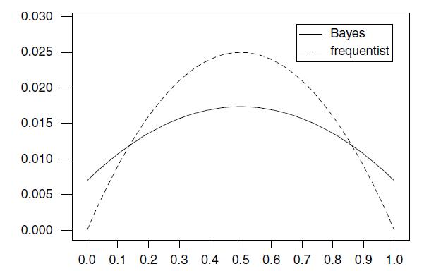ii. Over what range of values does the Bayesian estimator have smaller mean squared error than that of the frequentist estimator?

Transcribed Image Text:

0.030 0.025 0.020 0.015 0.010 0.005 0.000 Bayes frequentist 0.0 0.1 0.2 0.3 0.4 0.5 0.6 0.7 0.8 0.9 1.0