Use the RTD data in Examples 16-1 and 16-2 to predict X_PFR, X_CSTR, X_LFR, X_T-I-S, X_seg and X_mm for the following elementary gas-phase reactions

a. A → B k = 0.1 min^–1
b. A → 2B k = 0.1 min^–1
c. 2A → B k = 0.1 min^–1 m³/kmol C_A0 = 1.0 kmol/m³
d. 3A → B k = 0.1 m⁶/kmol²min C_A0 = 1.0 kmol/m³
Repeat (a) through (d) for the RTD given by
e. Problem P16-3B

Problem P16-3B

Consider the E(t) curve below.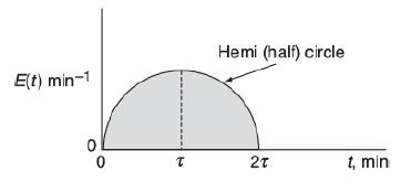

A graph is shown, with t (in minutes) on horizontal axis and E of t (minutes inverse) on vertical axis. A hemi (half) circular curve starts at the origin and ends at 2 tau on the horizontal axis. It is symmetric about the vertical line at tau. Mathematically this hemi circle is described by these equations: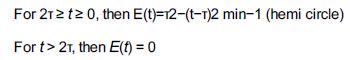

a. What is the mean residence time?
b. What is the variance?

f. Problem P16-4B

Problem P16-4B

A step tracer input was used on a real reactor with the following results: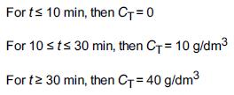

a. What is the mean residence time tm?
b. What is the variance σ²?

g. Problem P16-5B

Problem P16-5B

The following E(t) curves were obtained from a tracer test on two tubular reactors in which dispersion is believed to occur.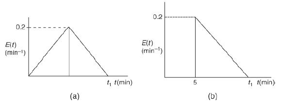

(a) RTD Reactor A; (b) RTD Reactor B The graphs for RTD reactors A and B are shown. The horizontal axis represents time (in minutes) and the vertical axis represents E of t (in minute inverse) in both graphs. The first graph is shown for RTD reactor A. The curve starts at the origin, increases linearly, reaches a maximum value of E of t at 0.2, and again gradually decreases to 0 at time interval t subscript 1. The second graph shows the response of RTD reactor B. The curve is a vertical line, where E(t) value increases from 0 to a maximum of 0.2 for the constant value 5 of t. After this, it linearly decreases and reaches 0 at t subscript 1.
a. What is the final time t1 (in minutes) for the reactor shown in Figure P16-5B (a)? How about in Figure P16-5B (b)?
b. What is the mean residence time, tm, and variance, =2, for the reactor shown in Figure P16-5B (a)? How about in Figure P16-5B (b)?
c. What is the fraction of the fluid that spends 7 minutes or longer in Figure P16-5B (a)? How about in Figure P16-5B (b)?

Examples 16-1

A sample of the tracer hytane at 320 K was injected as a pulse into a reactor, and the effluent concentration was measured as a function of time, resulting in the data shown in Table E16-1.1.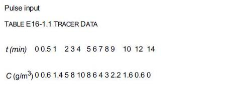

The measurements represent the exact concentrations at the times listed and not average values between the various sampling tests.
1. Construct a figure showing the tracer concentration C(t) as a function of time.
2. Construct a figure showing E(t) as a function of time.

Examples 16-2

Using the data given in Table E16-1.3 in Example 16-1
1. Construct the F(t) curve.
2. Calculate the mean residence time, tm.
3. Calculate the variance about the mean, σ2.
4. Calculate the fraction of fluid that spends between 3 and 6 minutes in the reactor.
5. Calculate the fraction of fluid that spends 2 minutes or less in the reactor.
6. Calculate the fraction of the material that spends 3 minutes or longer in the reactor.

Transcribed Image Text:

E(t) min-1 0 T Hemi (half) circle 20 t, min