Consider Private Equipment Company (PEC). On April 19, the PEC April 49 call option had a closing value of $4. The stock itself was selling at $50. On April 19, the option had 199 days to expiration (maturity date = November 4). The annual risk-free interest rate, continuously compounded, was 7 percent.

This information defines three variables directly:

1. The stock price, S, is $50.

2. The exercise price, E, is $49.

3. The risk-free rate, R, is .07.

In addition, the time to maturity, t, can be calculated quickly: The formula calls for t to be expressed in years.

4. We express the 199-day interval in years as t = 199 / 365.

In the real world, an option trader would know S and E exactly. Traders generally view U.S.

Treasury bills as riskless, so a current quote from www.bloomberg.com, or a similar source, would be obtained for the interest rate. The trader also would know (or could count) the number of days to expiration exactly. The fraction of a year to expiration, t, could be calculated quickly. The problem comes in determining the variance of the stock’s return. The formula calls for the variance between the purchase date of April 19 and the expiration date. Unfortunately, this represents the future, so the correct value for variance is not available. Instead, traders frequently estimate variance from past data, just as we calculated variance in an earlier chapter.

In addition, some traders may use intuition to adjust their estimate. For example, if anticipation of an upcoming event is likely to increase the volatility of the stock, the trader might adjust her estimate of variance upward to reflect this. (This problem was severe during and after the recession of 2008. The stock market was quite risky in the aftermath, so estimates using pre-recession data were too low.)

The preceding discussion was intended merely to mention the difficulties in variance estimation, not to present a solution. For our purposes, we assume that a trader has come up with an estimate of variance:

5. The variance of PEC stock has been estimated to be .09 per year.

Using these five parameters, we calculate the Black-Scholes value of the PEC call option in three steps:

Step 1: Calculate d1 and d2. These values can be determined by a straightforward, albeit tedious, insertion of our parameters into the basic formula. We have:

Step 2: Calculate N ( d 1 ) and N ( d 2 ) . We can best understand the values N ( d 1 ) and N ( d 2 ) by examining Figure 22.10. The figure shows the normal distribution with an expected value of 0 and a standard deviation of 1. This is frequently called the standard normal distribution. We mentioned in an earlier chapter that the probability that a drawing from this distribution will be between −1 and +1 (within one standard deviation of its mean) is 68.26 percent.

Now let us ask a different question: What is the probability that a drawing from the standardized normal distribution will be below a particular value? The probability that a drawing will be below 0 is clearly 50 percent because the normal distribution is symmetric. Using statistical Figure 22.10 Graph of Cumulative Probability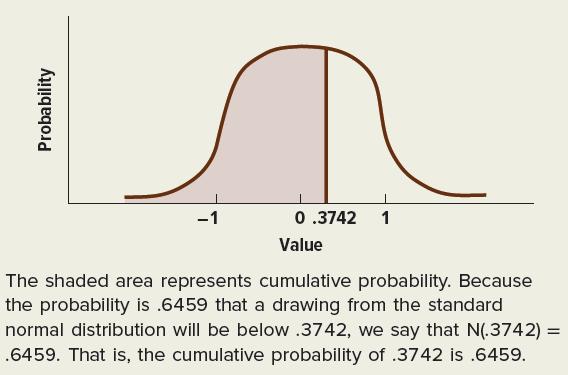

terminology, we say that the cumulative probability of 0 is 50 percent. Statisticians also say that N(0) = 50 percent. It turns out that:

The first value means that there is a 64.59 percent probability that a drawing from the standardized normal distribution will be below .3742. The second value means that there is a 56.07 percent probability that a drawing from the standardized normal distribution will be below .1527.

More generally, N ( d ) is the probability that a drawing from the standardized normal distribution will be below d. In other words, N ( d ) is the cumulative probability of d. Note that d 1 and d 2 in our example are slightly above zero, so N ( d 1 ) and N ( d 2 ) are slightly greater than .50.

Perhaps the easiest way to determine N ( d 1 ) and N ( d 2 ) is from the Excel function NORMSDIST.

In our example, NORMSDIST(.3742) and NORMSDIST(.1527) are .6459 and .5607, respectively.

We also can determine the cumulative probability from Table 22.3. Consider d = .37. This can be found in the table as .3 on the vertical and .07 on the horizontal. The value in the table Table 22.3 Cumulative Probabilities of the Standard Normal Distribution Function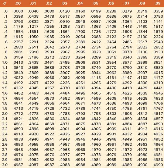

for d = .37 is .1443. This value is not the cumulative probability of .37. We must first make an adjustment to determine cumulative probability. That is:

Unfortunately, our table handles only two significant digits, whereas our value of .3742 has four significant digits. Hence, we must interpolate to find N(.3742). Because N(.37) = .6443 and N(.38) = .6480 , the difference between the two values is .0037 (= .6480 − .6443) . Because .3742 is 42 percent of the way between .37 and .38, we interpolate as:

The estimated price of $5.85 is greater than the $4 actual price, implying that the call option is underpriced. A trader believing in the Black-Scholes model would buy a call. Of course, the Black-Scholes model is fallible. Perhaps the disparity between the model’s estimate and the market price reflects error in the trader’s estimate of variance.

Transcribed Image Text:

d₁ = [In (§ ) + (R + 0²/2)t] / √o²t = [In (50)+(.07 + .09/2)× /1/.09 x 1991 365 V = [.0202 + .0627]/.2215 = .3742 d₂=d₁ - √o²t = .1527 a 199 365