In this exercise, we will derive the graph convolutional networks shown in Sec. 10.5.2 from spectral graph signal processing perspective. The classic convolution on graphs can be computed by $y=U{g}_{\theta }\left(\Lambda \right)U^{T}x$ where $x\in R^N$ is the input graph signal (i.e., a vector of scalars that denote feature values of all nodes at a certain feature dimension). Matrices $U$ and $\Lambda$ denote the eigen-decomposition of the normalized graph Laplacian: $L=I-D^{-\frac{1}{2}}A{D}^{-\frac{1}{2}}=U\Lambda U^T$. $g_{\theta }\left(\Lambda \right)$ is the function of eigenvalues and is often used as the filter function.

a. If we directly use the classic graph convolution formula where $g_{\theta }\left(\Lambda \right)=\mathrm{diag}\left(\theta \right)$ and $\theta \in$ $R^N$ to compute the output $y$, what are the potential disadvantages?

b. Suppose we use $K$-polynomial filter $g_{\theta }\left(\Lambda \right)={\sum }_{k=0}^K{\theta }_k{\Lambda }^k$. What are the benefits, compared to the above filter $g_{\theta }\left(\Lambda \right)=\mathrm{diag}\left(\theta \right)$ ?

c. By applying the $K$ th order Chebyshev polynomial approximation on the filter $g_{\theta }\left(\Lambda \right)=$ ${\sum }_{k=0}^K{\theta }_k{\Lambda }^k$, the filter function can be written as $g_{{\theta }^{\prime }}\left(\Lambda \right)\approx {\sum }_{k=0}^K{\theta }_k^{\prime }{T}_k\left(\tilde{\Lambda }\right)$ with a rescaled $\tilde{\Lambda }=\frac{2}{{\lambda }_{max}}\Lambda -I$, where ${\lambda }_{max}$ denotes the largest eigenvalue of $L$, and ${\theta }^{\prime }\in R^K$ denotes the Chebyshev coefficients. The Chebyshev polynomials can be computed recursively by $T_k\left(z\right)=2z{T}_{k-1}\left(z\right)-T_{k-2}\left(z\right)$ with $T_0\left(z\right)=1$ and $T_1\left(z\right)=\mathrm{Transcribed\; Image\; Text:}$

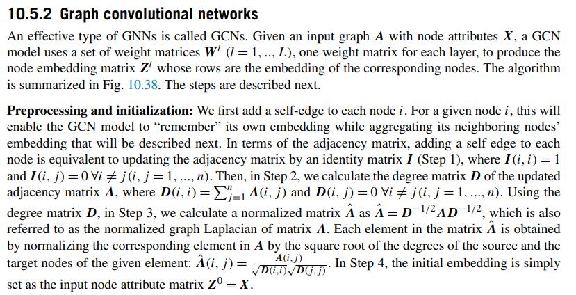
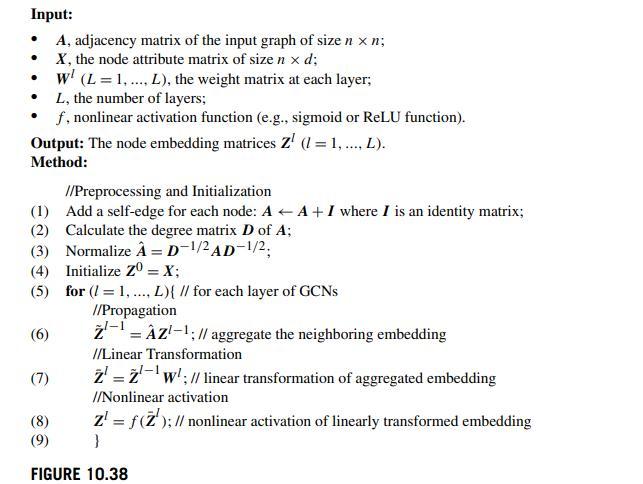
10.5.2 Graph convolutional networks An effective type of GNNs is called GCNs. Given an input graph A with node attributes X, a GCN model uses a set of weight matrices WI (l= 1,.., L), one weight matrix for each layer, to produce the node embedding matrix Z whose rows are the embedding of the corresponding nodes. The algorithm is summarized in Fig. 10.38. The steps are described next. Preprocessing and initialization: We first add a self-edge to each node i. For a given node i, this will enable the GCN model to "remember" its own embedding while aggregating its neighboring nodes' embedding that will be described next. In terms of the adjacency matrix, adding a self edge to each node is equivalent to updating the adjacency matrix by an identity matrix I (Step 1), where I (i, i) = 1 and I (i, j) = 0 Vi # j (i, j = 1, ..., n). Then, in Step 2, we calculate the degree matrix D of the updated adjacency matrix A, where D(i, i) =E=1 A(i, j) and D(i, j)=0 Vi j (i, j = 1, ..., n). Using the degree matrix D, in Step 3, we calculate a normalized matrix as = D-/2 AD-1/2, which is also referred to as the normalized graph Laplacian of matrix A. Each element in the matrix is obtained by normalizing the corresponding element in A by the square root of the degrees of the source and the A(i, j) target nodes of the given element: (i, j): D(ii) Dj.j)* D.). In Step 4, the initial embedding is simply = set as the input node attribute matrix Z = X.