Suppose we want to understand the demand curve for fish. We'll use the following demand curve equation:

Question:

\[ \text { Quantity }_{t}^{D}=\beta_{0}+\beta_{1} \text { Price }_{t}+\epsilon_{t}^{D} \]

Economic theory suggests \(\beta_{1}

(a) To see that prices and quantities are endogenous, draw supply and demand curves and discuss what happens when the demand curve shifts out (which corresponds to a change in the error term of the demand function). Note also what happens to price in equilibrium and discuss how this event creates endogeneity.

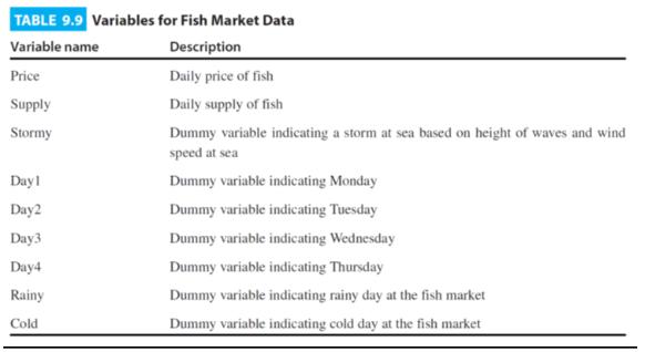
(b) The data set fishdata.dta (from Angrist, Graddy, and Imbens 2000) provides data on prices and quantities of a certain kind of fish (called whiting) over 111 days at the Fulton Street Fish Market, which then existed in Lower Manhattan. The variables are indicated in Table 9.9. The price and quantity variables are logged. Estimate a naive OLS model of demand in which quantity is the dependent variable and price is the independent variable. Briefly interpret results, and then discuss whether this analysis is useful.

(c) Angrist, Graddy, and Imbens suggest that a dummy variable indicating a storm at sea is a good instrumental variable that should affect the supply equation but not the demand equation. Stormy is a dummy variable that indicates a wave height greater than 4.5 feet and wind speed greater than 18 knots. Use 2SLS to estimate a demand function in which Stormy is an instrument for Price. Discuss first-stage and second-stage results, interpreting the most relevant portions.

(d) Reestimate the demand equation but with additional controls. Continue to use Stormy as an instrument for price, but now also include covariates that account for the days of the week and the weather on shore. Discuss firststage and second-stage results, interpreting the most relevant portions.

image text in transcribed