To find out who has a bank account (checking, savings, etc.) and who doesn€™t, John Caskey and Andrew Peterson estimated a probit model for the years 1977 and 1989, using data on U.S. households. The results are given in Table 15.25. The values of the slope coefficients given in the table measure the implied effect of a unit change in a regressor on the probability that a household has a bank account, these marginal effects being calculated at the mean values of the regressors included in the model.

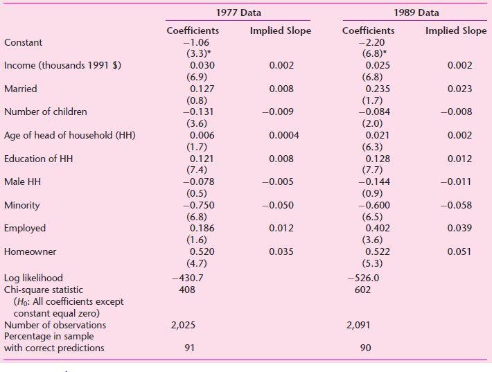
a. For 1977, what is the effect of marital status on ownership of a bank account? And for 1989? Do these results make economic sense?

b. Why is the coefficient for the minority variable negative for both 1977 and 1989?

c. How can you rationalize the negative sign for the number of children variable?

d. What does the chi-square statistic given in the table suggest?

Transcribed Image Text:

1977 Data 1989 Data Coefficients Implied Slope Coefficients Implied Slope -1.06 (3.3)* -2.20 (6.8)* Constant Income (thousands 1991 $) 0.030 0.002 0.025 0.002 (6.8) (6.9) Married 0.127 0.008 0.235 0.023 (0.8) -0.131 (1.7) -0.084 (2.0) Number of children -0.009 -0.008 (3.6) Age of head of household (HH) 0.0004 0.006 0.021 0.002 (1.7) (6.3) Education of HH 0.008 0.012 0.121 0.128 (7.7) (7.4) Male HH -0.078 -0.005 -0.144 -0.011 (0.5) (0.9) Minority -0.750 -0.050 -0.600 -0.058 (6.8) (6.5) 0.402 (3.6) Employed 0.012 0.186 0.039 (1.6) Homeowner 0.520 0.035 0.522 0.051 (4.7) (5.3) Log likelihood Chi-square statistic (Họ: All coefficients except constant equal zero) Number of observations -430.7 -526.0 408 602 2,025 2,091 Percentage in sample with correct predictions 91 90