The race track is a fascinating example of financial market dynamics at work. Let's go to the track and make a wager. Suppose that, from a field of 10 horses, we simply want to pick a winner. In the context of regression, we will let \(y\) be the response variable indicating whether a horse wins \((y=1)\) or not \((y=0)\). From racing forms, newspapers and so on, there are many explanatory variables that are publicly available that might help us predict the outcome for \(y\). Some candidate variables may include the age of the horse, recent track performance of the horse and jockey, pedigree of the horse, and so on. These variables are assessed by the investors present at the race, the betting crowd. Like many financial markets, it turns out that one of the most useful explanatory variable is the crowd's overall assessment of the horse's abilities. These assessments are not made from a survey of the crowd but rather from the wagers placed. Information about the crowd's wagers is available on a large sign at the race called the tote board. The tote board provides the odds of each horse winning a race. Table 11.12 is a
hypothetical tote board for a race of 10 horses.

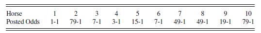
The odds that appear on the tote board have been adjusted to provide a " tracktake." That is, for every dollar that has been wagered, \(\$ T\) goes to the track for sponsoring the race and \(\$(1-T)\) goes to the winning bettors. Typical track takes are in the neighborhood of \(20 \%\), or \(T=0.20\).
We can readily convert the odds on the tote board to the crowd's assessment of the probabilities of winning. To illustrate this, Table 11.13 shows hypothetical bets to win which resulted in the displayed information on the hypothetical tote board in Table 11.12.

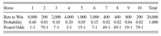
For this hypothetical race, \(\$ 20,000\) was bet to win. Because \(\$ 8,000\) of this \(\$ 20,000\) was bet on the first horse, interpret the ratio \(8,000 / 20,000=\) 0.40 as the crowd's assessment of the probability to win. The theoretical odds are calculated as \(0.4 /(1-0.4)=2 / 3\), or a 0.67 bet wins \(\$ 1\). However, the theoretical odds assume a fair game with no track take. To adjust for the fact that only \(\$(1-\mathrm{T})\) are available to the winner, the posted odds for this horse would be \(0.4 /(1-T-0.4)=1\), if \(T=0.20\). For this case, it now takes a \(\$ 1\) bet to win \(\$ 1\). We then have the relationship adjusted odds \(=x /(1-T-x)\), where \(x\) is the crowd's assessment of the probability of winning.
Before the start of the race, the tote board provides us with adjusted odds that can readily be converted into \(x\), the crowd's assessment of winning. We use this measure to help us to predict \(y\), the event of the horse actually winning the race.
We consider data from 925 races run in Hong Kong from September 1981 through September 1989. In each race, there were ten horses, one of which was randomly selected to be in the sample. In the data, use FINISH \(=y\) to be the indicator of a horse winning a race and WIN \(=x\) to be the crowd's a priori probability assessment of a horse winning a race.
a. A statistically naive colleague would like to double the sample size
by picking two horses from each race instead of randomly selecting one horse from a field of ten.

i. Describe the relationship between the dependent variables of the two horses selected.
ii. Say how this violates the regression model assumptions.
b. Calculate the average FINISH and summary statistics for WIN. Note that the standard deviation of FINISH is greater than that of WIN, even though the sample means are about the same. For the variable FINISH, what is the relationship between the sample mean and standard deviation?
c. Calculate summary statistics of WIN by level of FINISH. Note that the sample mean is larger for horses that won (FINISH \(=1\) ) than for those that lost \((\mathrm{FINISH}=0)\). Interpret this result.
d. Estimate a linear probability model, using WIN to predict FINISH.
i. Is WIN a statistically significant predictor of FINISH?
ii. How well does this model fit the data using the usual goodnessof-fit statistic?
iii. For this estimated model, is it possible for the fitted values to lie outside the interval \([0,1]\) ? Note, by definition, that the \(x\)-variable WIN must lie within the interval \([0,1]\).
e. Estimate a logistic regression model, using WIN to predict FINISH. Is WIN a statistically significant predictor of FINISH?
f. Compare the fitted values from the models in parts (d) and (e)
i. For each model, provide fitted values at WIN \(=0,0.01,0.05,0.10\), and 1.0 .
ii. Plot fitted values from the linear probability model versus fitted values from the logistic regression model.
g. Interpret WIN as the crowd's prior probability assessment of the probability of a horse winning a race. The fitted values, FINISH, is your new estimate of the probability of a horse winning a race, based on the crowd's assessment.
i. Plot the difference FINISH - WIN versus WIN.
ii. Discuss a betting strategy that you might employ based on the difference, FINISH - WIN.

Transcribed Image Text:

Horse 1 2 3 4 5 6 7 8 9 10 Posted Odds 1-1 79-1 7-1 3-1 15-1 7-1 49-1 49-1 19-1 79-1