The Capital Asset Pricing Model (CAPM) of W.F. Sharpe (1990 Nobel Prize in Economics) is based on a linear decomposition
\[
\frac{d S_{t}}{S_{t}}=(r+\alpha) d t+\beta \times\left(\frac{d M_{t}}{M_{t}}-r d tight)
\]
of stock returns \(d S_{t} / S_{t}\) into:
- a risk-free interest rate \(^{\frac{\ddagger}{+}} r\),
- an excess return \(\alpha\),
- a risk premium given by the difference between a benchmark market index return \(d M_{t} / M_{t}\) and the risk free rate \(r\).
The coefficient \(\beta\) measures the sensitivity of the stock return \(d S_{t} / S_{t}\) with respect to the market index returns \(d M_{t} / M_{t}\). In other words, \(\beta\) is the relative volatility of \(d S_{t} / S_{t}\) with respect to \(d M_{t} / M_{t}\), and it measures the risk of \(\left(S_{t}ight)_{t \in \mathbb{R}_{+}}\)in comparison to the market index \(\left(M_{t}ight)_{t \in \mathbb{R}_{+}}\).

If \(\beta>1\), resp. \(\beta
Vanguard 500 Index Fund (VFINX) has a \(\beta=1\) and can be considered as replicating the variations of the S\&P 500 index \(M_{t}\), while Invesco \(S \mathcal{E} P 500\) (SPHB) has a \(\beta=1.42\), and Xtrackers Low Beta High Yield Bond ETF (HYDW) has a \(\beta\) close to 0.36 and \(\alpha=6.36\).
In what follows, we assume that the benchmark market is represented by an index fund \(\left(M_{t}ight)_{t \in \mathbb{R}_{+}}\)whose value is modeled according to
\[
\begin{equation*}
\frac{d M_{t}}{M_{t}}=\mu d t+\sigma_{M} d B_{t} \tag{7.51}
\end{equation*}
\]
where \(\left(B_{t}ight)_{t \in \mathbb{R}_{+}}\)is a standard Brownian motion. The asset price \(\left(S_{t}ight)_{t \in \mathbb{R}_{+}}\)is modeled in a stochastic version of the CAPM as
\[
\begin{equation*}
\frac{d S_{t}}{S_{t}}=r d t+\alpha d t+\beta\left(\frac{d M_{t}}{M_{t}}-r d tight)+\sigma_{S} d W_{t} \tag{7.52}
\end{equation*}
\]

with an additional stock volatility term \(\sigma_{S} d W_{t}\), where \(\left(W_{t}ight)_{t \in \mathbb{R}_{+}}\)is a standard Brownian motion independent of \(\left(B_{t}ight)_{t \in \mathbb{R}_{+}}\), with
\[
\operatorname{Cov}\left(B_{t}, W_{t}ight)=0 \quad \text { and } \quad d B_{t} \cdot d W_{t}=0, \quad t \geqslant 0 .
\]
The following 10 questions are interdependent and should be treated in sequence.
a) Show that \(\beta\) coincides with the regression coefficient
\[
\beta=\frac{\operatorname{Cov}\left(d S_{t} / S_{t}, d M_{t} / M_{t}ight)}{\operatorname{Var}\left[d M_{t} / M_{t}ight]}
\]
Hint: We have
\[
\operatorname{Cov}\left(d W_{t}, d W_{t}ight)=d t, \quad \operatorname{Cov}\left(d B_{t}, d B_{t}ight)=d t, \quad \text { and } \quad \operatorname{Cov}\left(d W_{t}, d B_{t}ight)=0
\]
b) Show that the evolution of \(\left(S_{t}ight)_{t \in \mathbb{R}_{+}}\)can be written as
\[
d S_{t}=(r+\alpha+\beta(\mu-r)) S_{t} d t+S_{t} \sqrt{\beta^{2} \sigma_{M}^{2}+\sigma_{S}^{2}} d Z_{t}
\]
where \(\left(Z_{t}ight)_{t \in \mathbb{R}_{+}}\)is a standard Brownian motion.

Hint: The standard Brownian motion \(\left(Z_{t}ight)_{t \in \mathbb{R}_{+}}\)can be characterized as the only continuous (local) martingale such that \(\left(d Z_{t}ight)^{2}=d t\), see e.g. Theorem 7.36 page 203 of Klebaner (2005).
From now on, we assume that \(\beta\) is allowed to depend locally on the state of the benchmark market index \(M_{t}\), as \(\beta\left(M_{t}ight), t \geqslant 0\).
c) Rewrite the equations (7.51)-(7.52) into the system
\[
\left\{\begin{array}{l}
\frac{d M_{t}}{M_{t}}=r d t+\sigma_{M} d B_{t}^{*} \\
\frac{d S_{t}}{S_{t}}=r d t+\sigma_{M} \beta\left(M_{t}ight) d B_{t}^{*}+\sigma_{S} d W_{t}^{*}
\end{array}ight.
\]
where \(\left(B_{t}^{*}ight)_{t \in \mathbb{R}_{+}}\)and \(\left(W_{t}^{*}ight)_{t \in \mathbb{R}_{+}}\)have to be determined explicitly.

d) Using the Girsanov Theorem 7.3, construct a probability measure \(\mathbb{P}^{*}\) under which \(\left(B_{t}^{*}ight)_{t \in \mathbb{R}_{+}}\)and \(\left(W_{t}^{*}ight)_{t \in \mathbb{R}_{+}}\)are independent standard Brownian motions.
Hint: Only the expression of the Radon-Nikodym density \(\mathrm{dP} \mathbb{P}^{*} / \mathrm{dP}\) is needed here.
e) Show that the market based on the assets \(S_{t}\) and \(M_{t}\) is without arbitrage opportunities.
f) Consider a portfolio strategy \(\left(\xi_{t}, \zeta_{t}, \eta_{t}ight)_{t \in[0, T]}\) based on the three assets \(\left(S_{t}, M_{t}, A_{t}ight)_{t \in[0, T]}\), with value
\[
V_{t}=\xi_{t} S_{t}+\zeta_{t} M_{t}+\eta_{t} A_{t}, \quad t \in[0, T]
\]
where \(\left(A_{t}ight)_{t \in \mathbb{R}_{+}}\)is a riskless asset given by \(A_{t}=A_{0} \mathrm{e}^{r t}\). Write down the self-financing condition for the portfolio strategy \(\left(\xi_{t}, \zeta_{t}, \eta_{t}ight)_{t \in[0, T]}\).
g) Consider an option with payoff \(C=h\left(S_{T}, M_{T}ight)\), priced as
\[
f\left(t, S_{t}, M_{t}ight)=\mathrm{e}^{-(T-t) r} \mathbb{E}^{*}\left[h\left(S_{T}, M_{T}ight) \mid \mathcal{F}_{t}ight], \quad 0 \leqslant t \leqslant T .
\]
Assuming that the portfolio \(\left(V_{t}ight)_{t \in[0, T]}\) replicates the option price process \(\left(f\left(t, S_{t}, M_{t}ight)ight)_{t \in[0, T]}\), derive the pricing PDE satisfied by the function \(f(t, x, y)\) and its terminal condition.
Hint: The following version of the Itô formula with two variables can be used for the function \(f(t, x, y)\), see \((4.26)\) :

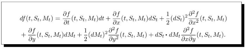
h) Find the self-financing hedging portfolio strategy \(\left(\xi_{t}, \zeta_{t}, \eta_{t}ight)_{t \in[0, T]}\) replicating the vanilla payoff \(h\left(S_{T}, M_{T}ight)\).
i) Solve the PDE of Question (g) and compute the replicating portfolio of Question (h) when \(\beta\left(M_{t}ight)=\beta\) is a constant and \(C\) is the European call option payoff on \(S_{T}\) with strike price \(K\).
j) Solve the PDE of Question (g) and compute the replicating portfolio of Question (h) when \(\beta\left(M_{t}ight)=\beta\) is a constant and \(C\) is the European put option payoff on \(S_{T}\) with strike price \(K\).

Transcribed Image Text:

df(t, St, Mt) + af at af (t, Si, Me)dM + =(aMe)2011 (t, St, Me) + dSe-dMe = af 1 of (t,St, Me)dSi + = (ds;)2021 -(t, St, Mt). 02 f (t, St, M)dt + 2 (t, St, Mt)