Consider the simple wage model in Example 10.2. Use the 428 observations on married women who participate in the labor force.

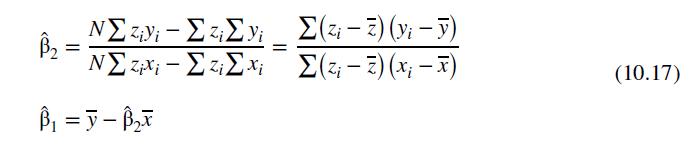
a. Using the instrumental variables estimator in equation (10.17), divide the numerator and denominator by \((N-1)\) and show that the IV estimator is the ratio of sample covariances, \(\hat{\beta}_{2}=\widehat{\operatorname{cov}}\left(z_{i}, y_{i}\right) / \widehat{\operatorname{cov}}\left(z_{i}, x_{i}\right)\).

b. Using your computer software, calculate \(\widehat{\operatorname{cov}}\left(\right.\) MOTHEREDUC \(\left.C_{i}, \ln \left(W A G E_{i}\right)\right)\) and \(\widehat{\operatorname{cov}}\left(\right.\) MOTHEREDUC \(\left._{i}, E D U C_{i}\right)\). Compare their ratio to the IV estimate in Example 10.2.

c. In Example 10.5, we added experience and its square to the model specification. To implement the ratio of covariances estimator in part (a), we first remove (partial-out) the influence of experience and its square from MOTHEREDUC, EDUC, and \(\ln (W A G E)\). Regress each of variables on EXPER and EXPER \({ }^{2}\) and save the residuals, calling them RMOTHEREDUC, REDUC, and RLWAGE. Calculate \(\widehat{\operatorname{cov}}\left(\right.\) RMOTHEREDUC \(_{i}\), RLWAGE \(\left._{i}\right)\) and \(\widehat{\operatorname{cov}}\left(\right.\) RMOTHEREDUC \(\left._{i}, R E D U C_{i}\right)\). Compare their ratio to the IV estimate in Example 10.5.

d. Using your IV/2SLS software, estimate the model \(R L W A G E=\beta_{2} R E D U C+\) error, omitting the constant term, using RMOTHEREDUC as an instrumental variable. Compare the resulting estimate to that in part (c).

Data From Example 10.5:-

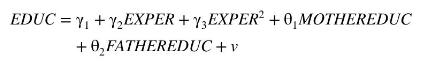
In addition to education a worker's experience is also important in determining their wage. Because additional years of experience have a declining marginal effect on wage use the quadratic model 

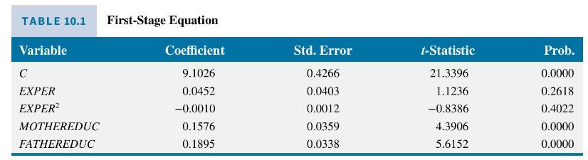
where EXPER is years of experience. This is the same specification. We assume that EXPER is an exogenous variable that is uncorrelated with the worker's ability and therefore uncorrelated with the random error \(e\). Two instrumental variables for years of education, \(E D U C\), are mother's and father's years of education, MOTHEREDUC and FATHEREDUC, introduced in the previous examples. The first-stage equation is  

Using the 428 observations in the data file mroz the estimated first-stage equation is reported in Table 10.1. The IV/2SLS estimates, with correctly computed standard errors, are

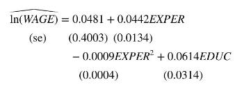
The estimated return to education is approximately \(6.1 \%\), and the estimated coefficient is statistically significant with a \(t=1.96\).

Data From Example 10.2:-

To illustrate the instrumental variables estimation method in a simple regression consider a simplified version of the model used in Example 10.1, \(\ln (W A G E)=\beta_{1}+\beta_{2} E D U C+e\). Using the data file mroz on \(N=428\) married women, the OLS estimates are

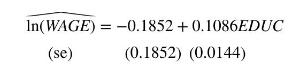
The estimated rate of return to education is approximately \(10.86 \%\), and \(t=7.55\) indicates that the estimated coefficient is significantly different from zero at even the \(1 \%\) level of significance. If \(E D U C\) is endogenous, and correlated with the random error \(e\), then OLS estimation may lead to incorrect inferences. We anticipate that \(E D U C\) is positively correlated with the omitted variable "ability," meaning that the estimated rate of return \(10.86 \%\) may overstate the true value.
What might we use as an instrumental variable? One proposal is to use mother's years of education, MOTHEREDUC, as an instrument. Does this qualify? In Section 10.3.3, we listed three criteria for an instrumental variable. First, does this variable have a direct effect on the dependent variable? Does it belong in the equation? Mother's education should not play any direct role in the determination of a daughter's wage, so this seems fine. Second, the instrument should not be contemporaneously correlated with the random error, \(e\). Is a mother's education correlated

with the omitted variable, her daughter's ability? This is more difficult. Ability includes many attributes, including intelligence, creativity, perseverance, and industriousness to name a few. Some portion of these character traits may be passed into our genetic makeup from our parents. We dodge the scientific debate on this issue and assume that a mother's years of education are uncorrelated with her daughter's ability. Third, the instrument should be highly correlated with the endogenous variable. This we can check! For the 428 women in the sample the correlation between mother's education and daughter's education is 0.3870 . This is not very large, but it is not very small either.
The instrumental variables estimates are

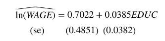
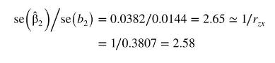
The IV estimate of the rate of return to education is \(3.85 \%\), one-third of the OLS estimate. The standard error is about 2.65 times larger than the OLS standard error, which is very close to what we reasoned that the ratio might be when both estimators are consistent,

Data From Equation 10.17:-

Transcribed Image Text:

In(WAGE) = B+ BEXPER+ BEXPER + BEDUC + e