In Appendix 16A.1, we illustrate the calculation of a standard error for the marginal effect in a probit model of transportation, Example 16.4. In the appendix, the calculation is for the marginal effect when it currently takes 20 minutes longer to commute by bus \((D T I M E=2)\).

a. Repeat the calculation for the probit model when DTIME \(=1\). 

b. Using the probit model, construct a \(95 \%\) interval estimate for the marginal effect of a 10-minute increase in travel time by bus when DTIME \(=1\).

c. The logit model estimates and standard errors are

\[\begin{gathered}\tilde{\gamma}_{1}+\tilde{\gamma}_{2} \text { DTIME }=-0.2376+0.5311 \text { DTIME } \\(\mathrm{se}) \quad(0.7505)(0.2064)\end{gathered}\]

The estimated coefficient covariance is \(\widehat{\operatorname{cov}}\left(\tilde{\gamma}_{1}, \tilde{\gamma}_{2}\right)=-0.025498\). Calculate the standard error of the marginal effect of a 10-minute increase in travel time when DTIME \(=1\). 

d. Construct a 95\% interval estimate for the marginal effect of a 10-minute increase in travel time by bus, when \(D T I M E=1\) for the logit model.

Data From Example 16.4:-

In Example 16.2, we estimated a linear probability model using the transportation data, transport. In this example, we carry out probit estimation. The probit model is \(P(A U T O=1)=\Phi\left(\beta_{1}+\beta_{2}\right.\) DTIME \()\). The maximum likelihood estimates of the parameters are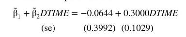

The values in parentheses below the parameter estimates are estimated standard errors that are valid in large samples. These standard errors can be used to carry out hypothesis tests and construct interval estimates in the usual way, with the qualification that they are valid in large samples. The negative sign of \(\tilde{\beta}_{1}\) implies that when commuting times via bus and auto are equal so \(D T I M E=0\), individuals have a bias against driving to work, relative to public transportation, The estimated probability of a person choosing to drive to work when DTIME \(=0\) is \(\hat{P}(A U T O=1 \mid D T I M E=0)=\Phi(-0.0644)=0.4743\). The positive sign of \(\tilde{\beta}_{2}\) indicates that an increase in public transportation travel time, relative to auto travel time, increases the probability that an individual will choose to drive to work, and this coefficient is statistically significant.
Suppose that we wish to estimate the marginal effect of increasing public transportation time, given that travel via public transportation currently takes 20 minutes longer than auto travel. Using (16.11),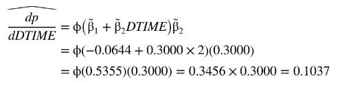

For the probit probability model, an incremental (10-minute) increase in the travel time via public transportation increases the probability of travel via auto by approximately 0.1037 , given that taking the bus already requires 20 minutes more travel time than driving.

The estimated parameters of the probit model can also be used to "predict" the behavior of an individual who must choose between auto and public transportation to travel to work. If an individual is faced with the situation that it takes 30 minutes longer to take public transportation than to drive to work, then the estimated probability that auto transportation will be selected is calculated using (16.12):
\[\begin{aligned}\hat{p} & =\Phi\left(\tilde{\beta}_{1}+\tilde{\beta}_{2} \text { DTIME }\right)=\Phi(-0.0644+0.3000 \times 3) \\& =0.7983\end{aligned}\]
Since the estimated probability that the individual will choose to drive to work is 0.7983 , which is greater than 0.5 , we "predict" that when public transportation takes 30 minutes longer than driving to work, the individual will choose to drive.

Data From Equation 16.12:-

Data From Example 16.2:-

Ben-Akiva and Lerman \({ }^{1}\) have sample data on automobile and public transportation travel times and the alternative chosen for \(N=21\) individuals in the data file transport. The variable \(A U T O\) is an indicator variable taking the value one if automobile transportation is chosen and is zero if public transportation is chosen,

The variables AUTOTIME and BUSTIME are minutes of commuting time. The explanatory variable we consider is DTIME \(=(\) BUSTIME - AUTOTIME \() \div 10\), which is the commuting time differential in 10 -minute increments. The linear probability model is AUTO \(_{i}=\beta_{1}+\beta_{2}\) DTIME \(_{i}+e_{i}\). The OLS fitted model, with heteroskedasticity robust standard errors, is
\[\begin{array}{lll}\widehat{A U T O}_{i}=0.4848+0.0703 D T I M E_{i} & R^{2}=0.61 \\\text { (robse) } \quad(0.0712)(0.0085) &\end{array}\]
We estimate that if travel times by public transportation and automobile are equal, so that DTIME \(=0\), then the probability of a person choosing automobile travel is 0.4848 , close to \(50-50\), with a \(95 \%\) interval estimate of [0.34, 0.63]. We estimate that, holding all else constant, an increase of 10 minutes in the difference in travel time, increasing public transportation travel time relative to automobile travel time, increases the probability of choosing automobile travel by 0.07 , with a \(95 \%\) interval estimate of \([0.0525,0.0881]\), which seems relatively precise. In truth, any judgment about precision depends on the use to which the results will be put. The fitted model can be used to estimate the probability of automobile travel for any commuting time differential. For example, if \(D T I M E=1\), a 10-minute longer commute by public transportation, we estimate the probability of automobile travel to be \(\widehat{A U T O}_{i}=0.4848+0.0703(1)=0.5551\).
How well does the model fit the data? The \(R^{2}=0.61\) suggests that \(61 \%\) of the variation in the outcome variable is explained by the model. With probability models, we can examine how well the model predicts the outcomes. Let's predict the choice using a probability threshold of 0.50 . That is, if \(\widehat{A U T O}_{i} \geq 0.50\) we predict that a person will drive to work, and otherwise, we predict that a person will use public transportation. In the sample of 21 individuals, 10 drove to work and 11 used public transportation. Using the classification rule, we successfully predict 9 of the 10 drivers, and 10 of the 11 bus riders. That is 19 successful predictions out of the 21 cases. Looking at individual estimated probabilities of driving, we find three negative values. If the commute is 69 minutes or less by public transportation, then the estimated probability of driving is zero or negative. If commuting time is 73 minutes or more by public transportation, then the estimated probability of driving is one or greater.

Transcribed Image Text:

B + BDTIME = 0.0644 +0.3000DTIME (se) (0.3992) (0.1029)