In Example 12.2, using data from the data file toody 5, we estimated the model

\[\ln \left(Y_{I E L D_{t}}\right)=\alpha_{1}+\alpha_{2} t+\beta_{1} \text { RAIN }_{t}+\beta_{2} \text { RAIN }_{t}^{2}+e_{t}\]

An assumption underlying this example was that \(\ln (Y I E L D), R A I N\), and RAIN \({ }^{2}\) are all trend stationary. Test this assumption using a 5\% significance level.

Data From Example 12.2:-

Scientists are continually working on ways to increase global food production to keep pace with a growing world population. One small contribution to this effort is the work of agronomists who develop new varieties of wheat to increase wheat yield. In the Toodyay Shire of Western Australia, we expect wheat yield to be trending upward over time reflecting the development of new varieties. However, wheat growing in Western Australia is a risky business. Its success depends heavily on rainfall, which is not always reliable.

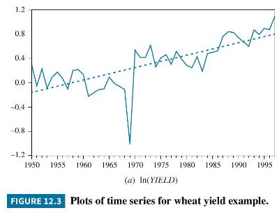
Thus, we expect yield to fluctuate around an increasing trend. Data on annual wheat yield and rainfall during the growing season for the Toodyay Shire, from 1950 to 1997, can be found in the data file toody5. For wheat yield, we use the constant growth rate trend \(\ln \left(Y I E L D_{t}\right)=a_{1}+a_{2} t+u_{t}\). The observations for \(\ln \left(Y I E L D_{t}\right)\) are plotted in Figure 12.3(a), along with the linear trend line. The observations fluctuate around the increasing trend with a particularly bad year in 1969. Examining the rainfall data in Figure 12.3(b), we

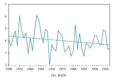
discover there is a slight downward trend and very little rainfall in 1969.
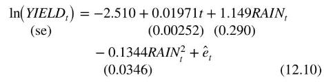
It turns out that there are decreasing returns to rainfall and so we include RAIN \({ }^{2}\) as well as RAIN in the model, leading to the following estimated equation

The other alternative is to detrend \(\ln (Y I E L D)\), RAIN, and \(R A I N^{2}\) and to estimate the detrended model. First, estimating the trends, we obtain

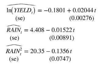
The first two equations describe the trend lines in Figure 12.3. After computing \(\operatorname{RRAIN}_{t}=R A I N_{t}-\widehat{R A I N}_{t}\), RRAIN \(_{t}=\) RAIN \(_{t}^{2}-\widehat{\text { RAIN }_{t}^{2}}\), and \(R L Y I E L D_{t}=\ln \left(Y_{I E L D}\right)-\) \(\widehat{\ln \left(\text { YIELD }_{t}\right)}\), we obtain

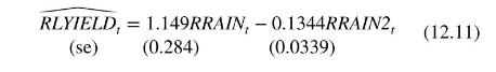
Notice the estimates in (12.10) and (12.11) are identical, but the standard errors are not. The standard error discrepancy arises from the different degrees of freedom used to estimate the error variance. In (12.10), it is \(48-4=44\); in (12.11), it is \(48-2=46\). We can correct the standard errors in (12.11) by multiplying them by \(\sqrt{46 / 44}=1.022\). In large samples, the difference will be negligible. The legitimacy of the estimates in (12.10) and (12.11) depends on the assumption that \(\ln (Y I E L D), R A I N\), and RAIN \({ }^{2}\) are trend stationary. This assumption can be checked using the hypothesis testing machinery that is developed in Section 12.3.

Transcribed Image Text:

1.2 0.8 0.4 0 0.0 -0.4 -0.8 -1.2 1950 1955 1960 1965 1970 1975 1980 1985 1990 1995 (a) In(YIELD) FIGURE 12.3 Plots of time series for wheat yield example.