Table 15.9 contains some simulated panel data, where \(i d\) is the individual cross-section identifier, \(t\) is the time period, \(x\) is an explanatory variable, \(e\) is the idiosyncratic error, \(y\) is the outcome value. The data generating process is \(y_{i t}=10+5 x_{i t}+u_{i}+e_{i t}, i=1,2,3, t=1,2\). The OLS residuals are \(\hat{e}\), which we have rounded to two decimal places for convenience.

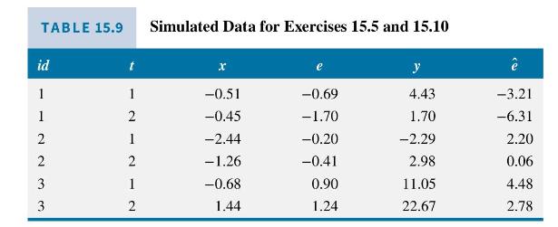
a. Using the true data generating process, calculate \(u_{i}, i=1,2,3\).

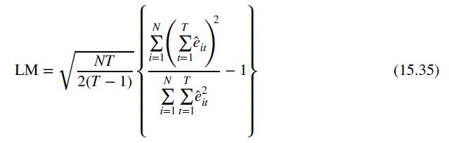
b. Calculate the value of the LM statistic in equation (15.35) and carry out a test for the presence of random effects at the \(5 \%\) level of significance.

c. The fixed effects estimate of the coefficient of \(x_{i t}\) is \(b_{F E}=5.21\) with standard error 0.94 , while the random effects estimate is \(b_{R E}=5.31\) with standard error 0.81 . Test for the presence of correlation between the unobserved heterogeneity \(u_{i}\) and the explanatory variable \(x_{i t}\). (Note: The sample is actually too small for this test to be valid.)

d. If estimates of the variance components are \(\hat{\sigma}_{u}^{2}=34.84\) and \(\hat{\sigma}_{e}^{2}=2.59\), calculate an estimated value of the GLS transformation parameter \(\alpha\). Based on its magnitude, would you expect the random effects estimates to be closer to the OLS estimates or the fixed effects estimates.

e. Using the estimates in (d), compute an estimate of the correlation between \(v_{i 1}=u_{i}+e_{i 1}\) and \(v_{i 2}=u_{i}+e_{i 2}\). Is this correlation relatively high, or relatively low?

Data From Equation 15.35:-

Transcribed Image Text:

TABLE 15.9 Simulated Data for Exercises 15.5 and 15.10 id y 1 1 -0.51 -0.69 4.43 -3.21 1 2 -0.45 -1.70 1.70 -6.31 2233 1 -2.44 -0.20 -2.29 2.20 2 3 212 -1.26 -0.41 2.98 0.06 -0.68 0.90 11.05 4.48 1.44 1.24 22.67 2.78