(a) Explain why, physically, when the Brownian motion of a particle (which starts at x = 0 at time t = 0) is observed only on timescales △τ >> τ_r corresponding to frequencies f r , its position x(t)must be a Gaussian-Markov process with x̄ = 0.What are the spectral density of x(t) and its relaxation time in this case?

(b) Use Doob’s theorem to compute the conditional probability P₂(x₂, τ |x₁). Your answer should agree with the result deduced in Ex. 6.3 from the diffusion equation, and in Ex. 6.4 from the central limit theorem for a random walk.

Data from Exercises 6.3

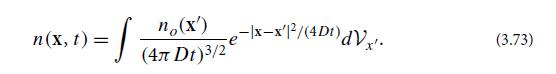
In Ex. 3.17, we studied the diffusion of particles through an infinite 3-dimensional medium. By solving the diffusion equation, we found that, if the particles’ number density at time t = 0 was n_o(x), then at time t it has become

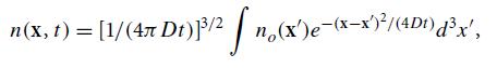
where D is the diffusion coefficient [Eq. (3.73)].

For any one of the diffusing particles, the location y(t) in the y direction (one of three Cartesian directions) is a 1-dimensional random process. From the above n(x, t), infer that the conditional probability distribution for y is

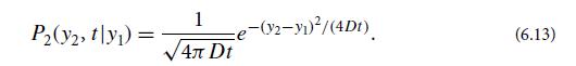
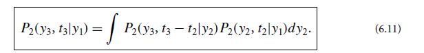
Verify that the conditional probability (6.13) satisfies the Smoluchowski equation (6.11).

At first this may seem surprising, since a particle’s position y is not Markov. However, the diffusion equation from which we derived this P₂ treats as negligibly small the timescale τ_r on which the velocity dy/dt thermalizes. It thereby wipes out all information about what the particle’s actual velocity is, making y effectively Markov, and forcing its P₂ to satisfy the Smoluchowski equation.

Data from Exercises 6.4

A particle travels in 1 dimension, along the y axis, making a sequence of steps △y_j (labeled by the integer j ), each of which is △y_j = +1 with probability 1/2, or △y_j = −1with probability 1/2.

After N >> 1 steps, the particle has reached location 

What does the central limit theorem predict for the probability distribution of y(N)? What are its mean and its standard deviation?

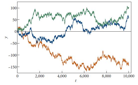
Viewed on length scales >> 1, y(N) looks like a continuous random process, so we shall rename N ≡ t . Using the (pseudo)random number generator from your favorite computer software language, compute a few concrete realizations of y(t) for 0 4 and plot them.⁴ Figure 6.1 above shows one realization of this random process.

Explain why this random process is Markov.

Use the central limit theorem to infer that the conditional probability P₂ for this random process is

Notice that this is the same probability distribution as we encountered in the diffusion exercise but with D = 1/2. Why did this have to be the case?

Using an extension of the computer program you wrote in part (b), evaluate y(t = 10⁴) for 1,000 realizations of this random process, each with y(0) = 0, then bin the results in bins of width δy = 10, and plot the number of realizations y(10⁴) that wind up in each bin. Repeat for 10,000 realizations. Compare your plots with the probability distribution (6.17).

Figure 6.1

Transcribed Image Text:

n(x, 1) = [1/(47 Dt)³/² [ n(x')e¯(x-x')²/(4D1) d³x', t)