Use Laplace-transform techniques to derive Eqs. (22.29)–(22.31) for the time evolving electric field of electrostatic waves with fixed wave number k and initial velocity perturbations F_s1(v, 0). A sketch of the solution follows.

(a) When the initial data are evolved forward in time, they produce Fs1(v, t) and E(t). Construct the Laplace transforms of these evolving quantities:

To ensure that the time integral is convergent, insist that R(p) be greater than

(the e-folding rate of the most strongly growing mode—or, if none grow, then the most weakly damped mode). Also, to simplify the subsequent analysis, insist that R(p) > 0.Below, in particular, we need the Laplace transforms for R(p) = (some fixed value σ that satisfies σ > p_o and σ > 0).

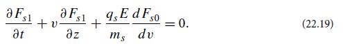
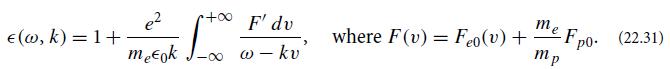
(b) By constructing the Laplace transform of the 1-dimensional Vlasov equation (22.19) and integrating by parts the term involving ∂F_s1/∂t, obtain an equation for a linear combination of F̃_s1(v, p) and Ẽ(p) in terms of the initial data F_s1(v, t = 0). By then combining with the Laplace transform of Poisson’s equation, show that

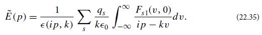
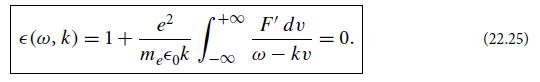
Here ∈(ip, k) is the dielectric function (22.25) evaluated for frequency ω = ip, with the integral running along the real v-axis, and [as we noted in part (a)] with R(p) greater than p₀, the largestωi of any mode, and greater than 0. This situation for the dielectric function is the one depicted in Fig. 22.2a.

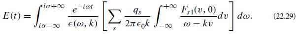
(c) Laplace-transform theory tells us that the time-evolving electric field (with wave number k) can be expressed in terms of its Laplace transform (22.35) by

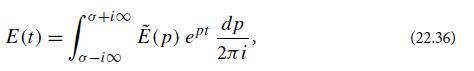
where σ [as introduced in part (a)] is any real number larger than p₀ and larger than 0. Combine this equation with expression (22.35) for Ẽ(p), and set p = −iω. Thereby arrive at the desired result, Eq. (22.29).

Equations.

Transcribed Image Text:

8 F₁1(v, p) = [ dt e-pt F(v, t), = 5₁°⁰ f Ē(p) = dt e-pt E (t). (22.34)