In this problem we derive and explore the theoretical and empirical implications of a lower bound on the forward-looking expected equity premium, derived by Martin (2017). The lower bound is the risk-neutral conditional variance of equity returns divided by the gross risk-free rate.

Martin (2017) introduces a volatility index, SVIX \({ }_{i, t, T}\), defined in terms of the time\(t\) prices of put and call options on an underlying asset or portfolio \(i\), usually a market index, with different strike prices and the same maturity \(T\). It turns out that the square of the SVIX equals the (normalized) risk-neutral conditional variance of the gross simple return \(R_{i, t, T}\) on the underlying asset \(i\),

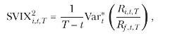
The asterisk denotes moments of the risk-neutral distribution of returns. The fact that SVIX is directly observable at time \(t\) from the cross section of option prices implies that the lower bound on the equity premium that we will derive below is directly observable. In general, moments of the risk-neutral (conditional) distribution of asset returns can be backed out from option prices.

(a) Show that

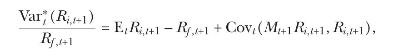
where \(M_{t+1}\) denotes the stochastic discount factor.
Conclude that \(\operatorname{Var}_{t}^{*}\left(R_{i, t+1}ight) / R_{f, t+1}=R_{f, t+1} \operatorname{SVIX}_{i, t+1}^{2}\) is a lower bound on the equity premium, \(\mathrm{E}_{t} R_{i, t+1}-R_{f, t+1}\), provided that the negative correlation condition,

(b) Although SVIX has not yet been put to practical use, a well-known volatility index that is closely related to the SVIX is the VIX. It turns out that the VIX satisfies

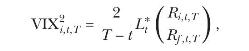
where \(L^{*}(\cdot)\) is the risk-neutral entropy of returns.
(i) What risk-neutral distribution of returns would approximately equate the VIX and the SVIX (for short maturities \(T\) )?
(ii) Assume that returns and the stochastic discount factor are jointly conditionally lognormal (with respect to the objective probability measure). Show that

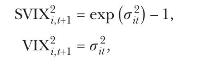
where \(\sigma_{i, t}^{2}\) is the conditional variance of \(r_{i, t+1}=\log R_{i, t+1}\). To derive the expression for the VIX you will need to make use of Stein's Lemma: if \(X\) and \(Y\) are two jointly normally distributed variables, \(\operatorname{Cov}(h(X), Y)=\mathrm{E}\left[h^{\prime}(X)ight] \operatorname{Cov}(X, Y)\), for any differentiable function \(h(\cdot)\) such that \(\mathrm{E}\left[h^{\prime}(X)ight]\) and \(\operatorname{Cov}(h(X), Y)\) exist.
(iii) In recent data the VIX is always higher than the SVIX. What does this tell us about the usual assumption of conditionally lognormal returns?

(c) We now investigate the theoretical relevance of the negative correlation condition. Take asset \(i\) to be the market portfolio of risky assets. Show whether or not (NCC) holds in each of the following settings, or whether additional assumptions need to be imposed:
(i) An economy where there exists an unconstrained risk-neutral investor.
(ii) An economy where there exists a CRRA agent who lives only for periods \(t\) and \(t+1\) and who holds the market.
(iii) An economy where the stochastic discount factor and the market return are conditionally jointly lognormal and where the market's conditional Sharpe ratio, \(\log \mathrm{E}_{t}\left[R_{m, t+1} / R_{f, t+1}ight] / \sigma_{t}\left(\log R_{m, t+1}ight)\), exceeds the conditional volatility of the market, \(\sigma_{t}\left(\log R_{m, t+1}ight)\).
In light of these results, do you think that (NCC) imposes rather strong or weak restrictions on preferences?

(d) Empirical estimates of \(\operatorname{Cov}_{t}\left(M_{t+1} R_{m, t+1}, R_{m, t+1}ight)\) in linear factor models are negative and close to zero. Indeed, the time-series average of the lower bound in recent data is around \(5 \%\), quite close to the typical estimates of the unconditional equity premium. If the lower bound is approximately satisfied with equality, what would this imply about the relative risk aversion of a marginal investor who holds the market? Consider, for example, the setting of part

(c) (ii).

(e) The risk-neutral variance (SVIX) approach presents an alternative to the large literature seeking to estimate the equity premium via predictive regressions based on valuation ratios discussed in this chapter. Compare and discuss the advantages and disadvantages of each approach.

(f) A notable divergence of forecasts between the risk-neutral variance approach and the valuation-ratios approach occurred in the late 1990s. The monthly and quarterly forecasts for the SVIX bound were high from late 1998 until the end of 1999, consistent with the high equity premia subsequently realized during that period. In contrast, valuation ratios were so low that predictive regressions forecasted a negative equity premium. Is it possible to reconcile these contrasting forecasts?
use the the Campbell-Shiller approximation to the dividend yield to think about what the dividend yield forecasts.

Transcribed Image Text:

SVIXT 1 Var (R) T-t