In heat transfer the heat transfer from a slab of thickness 2w initially at a uniform temperature T₀ can sometimes be modeled by a lumped parameter analysis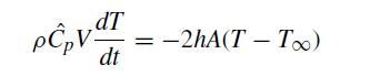

where ρ is the density of the slab, Cˆp is its heat capacity, h is the heat transfer coefficient, and T_∞ is the temperature far from the slab. The volume of the slab is V = 2wA, where A is the surface area of one face. The factor of 2 appears in the equation because there are two faces. The solution to this problem is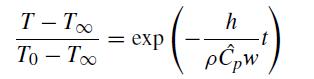

If we define the dimensionless temperature θ ≡ (T − T∞)/(T₀ − T_∞) and the dimensionless time τ = ht/ρ Cˆ_pw, then the lumped parameter solution is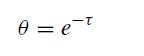

Here, we will consider the accuracy of this approximation as a function of the Biot number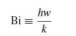

where k is the thermal conductivity of the slab. The unsteady heat equation is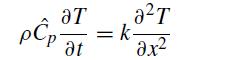

If the initial condition is uniform, T(x, 0) = T0, then the problem is symmetric about x = 0 and we can solve it subject to the symmetry boundary condition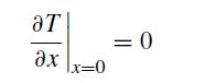

and the heat transfer boundary condition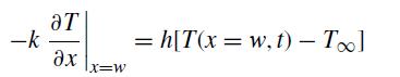

If we use the same dimensionless time and temperature, and introduce a dimensionless position z = x/w, then the differential equation becomes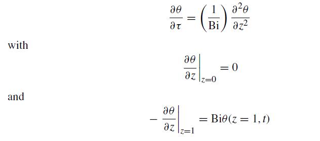

(a) Write a MATLAB program that uses the method of lines and finite differences to solve this equation, where you do the time integration using RK4. Include the system of ODEs that you need to solve at each step. Have your program integrate out to a dimensionless time of τ = 0.001 using a grid spacing Δz = 0.005 and time step h = 10⁻⁴. Your program should automatically plot the temperature profile at the final time for Bi = 1000, 50, 20, 10, 5, and 1 as separate figures. Include an explanation for their behavior.

(b) You should notice that the solution in part (a) is not very good. (Indeed, since this linear problem has a solution by separation of variables, our numerical solution so far is a waste of time!) Rewrite your program to solve the problem using implicit Euler as the integration method, and include the details of the integration scheme in your written solution. This time, have your program integrate out to τ = 0.5 for Bi = 0.01, 1, 5, 10, 50, and 1000. Your program should automatically generate a plot of the temperature profile for all of the Bi numbers on a single graph, which should also have the prediction from the lumped parameter analysis too. Include an explanation of what is going on.

Transcribed Image Text:

pCp T dt = -2hA(T-Too)