

1) Suppose there is a service center consisting of a single server. Let the external arrival...
Fantastic news! We've Found the answer you've been seeking!
Question:
Transcribed Image Text:
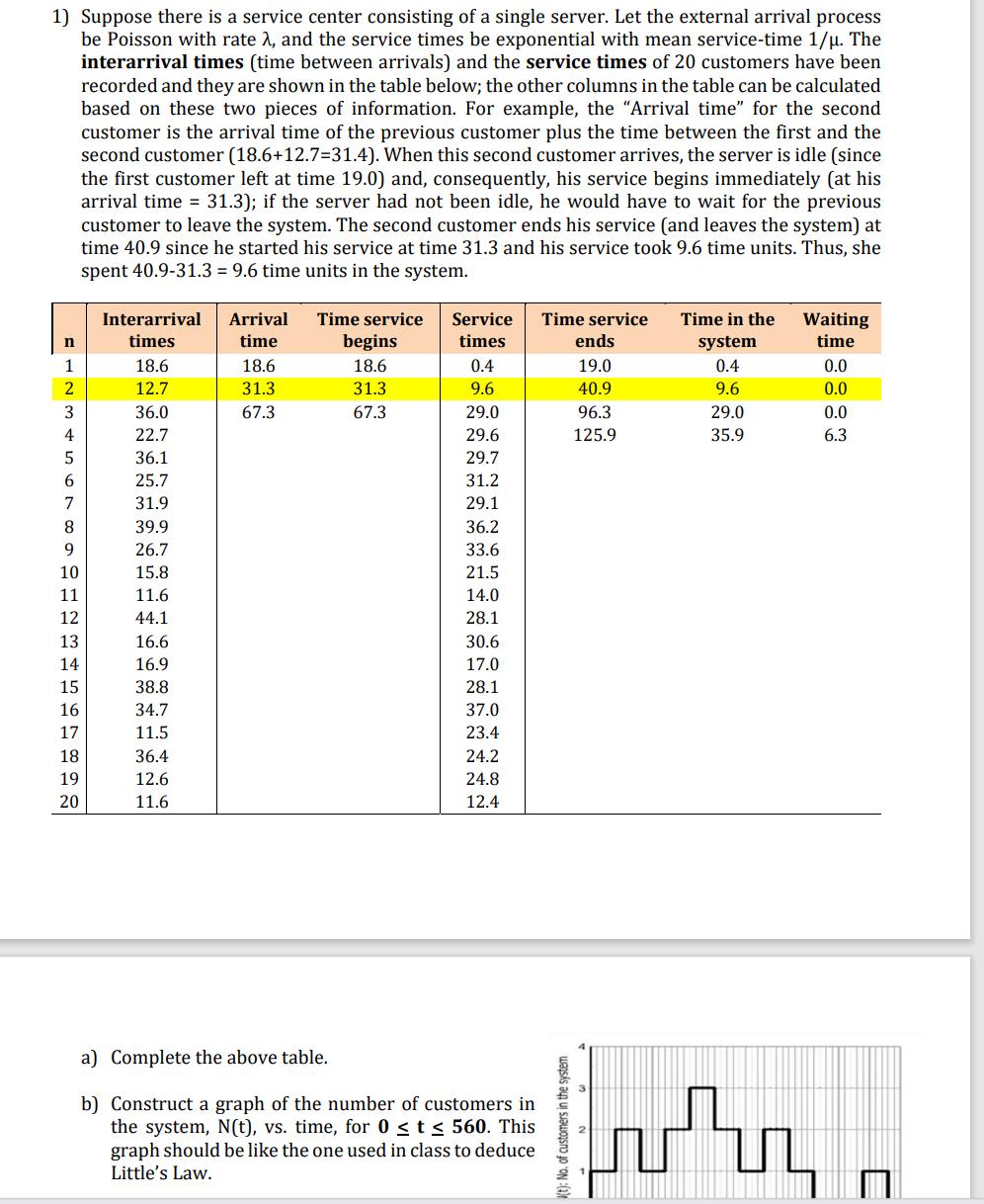
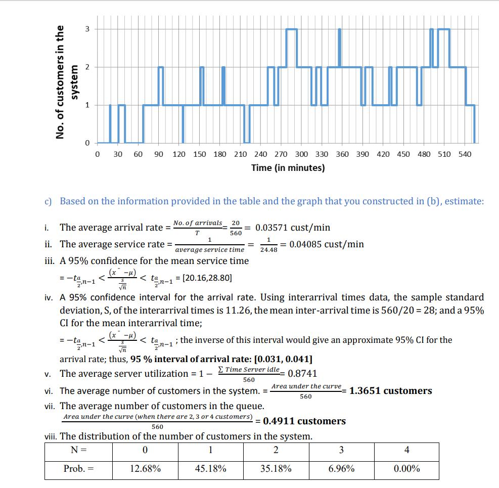
1) Suppose there is a service center consisting of a single server. Let the external arrival process be Poisson with rate λ, and the service times be exponential with mean service-time 1/μ. The interarrival times (time between arrivals) and the service times of 20 customers have been recorded and they are shown in the table below; the other columns in the table can be calculated based on these two pieces of information. For example, the "Arrival time" for the second customer is the arrival time of the previous customer plus the time between the first and the second customer (18.6+12.7-31.4). When this second customer arrives, the server is idle (since the first customer left at time 19.0) and, consequently, his service begins immediately (at his arrival time = 31.3); if the server had not been idle, he would have to wait for the previous customer to leave the system. The second customer ends his service (and leaves the system) at time 40.9 since he started his service at time 31.3 and his service took 9.6 time units. Thus, she spent 40.9-31.3 = 9.6 time units in the system. n 1 2 3 4 5 6 7 8 9 10 U 11 12 13 14 15 16 17 18 19 20 Interarrival times 18.6 12.7 36.0 22.7 36.1 25.7 31.9 39.9 26.7 15.8 11.6 44.1 16.6 16.9 38.8 34.7 11.5 36.4 12.6 11.6 Arrival time 18.6 31.3 67.3 Time service Service times begins 18.6 31.3 67.3 0.4 9.6 29.0 29.6 29.7 31.2 29.1 36.2 33.6 21.5 14.0 28.1 30.6 17.0 28.1 37.0 23.4 24.2 24.8 12.4 a) Complete the above table. b) Construct a graph of the number of customers in the system, N(t), vs. time, for 0 ≤ t ≤ 560. This graph should be like the one used in class to deduce Little's Law. Time service Time in the system 0.4 9.6 (t): No. of customers in the system ends 19.0 40.9 96.3 125.9 29.0 35.9 Waiting time ц 0.0 0.0 0.0 6.3 No. of customers in the system 0 30 60 90 120 150 180 210 240 270 300 330 360 390 420 450 480 510 540 Time (in minutes) c) Based on the information provided in the table and the graph that you constructed in (b), estimate: No. of arrivals 20 560 i. The average arrival rate = = -t T 1 ii. The average service rate = average service time iii. A 95% confidence for the mean service time (x-μ) = 0.03571 cust/min 1 24.48 tn-1=[20.16,28.80] √n iv. A 95% confidence interval for the arrival rate. Using interarrival times data, the sample standard deviation, S, of the interarrival times is 11.26, the mean inter-arrival time is 560/20 = 28; and a 95% CI for the mean interarrival time; <ta ; the inverse of this interval would give an approximate 95% CI for the = 0.04085 cust/min 45.18% (x-μ). = tan-1 √n arrival rate; thus, 95 % interval of arrival rate: [0.031, 0.041] Σ Time Server idle- 0.8741 The average server utilization = 1 - 560 v. vi. The average number of customers in the system. = vii. The average number of customers in the queue. Area under the curve (when there are 2, 3 or 4 customers) 560 viii. The distribution of the number of customers in the system. N = 0 2 Prob. = 12.68% 35.18% Area under the curve- 1.3651 customers 560 = 0.4911 customers 3 6.96% 0.00% 1) Suppose there is a service center consisting of a single server. Let the external arrival process be Poisson with rate λ, and the service times be exponential with mean service-time 1/μ. The interarrival times (time between arrivals) and the service times of 20 customers have been recorded and they are shown in the table below; the other columns in the table can be calculated based on these two pieces of information. For example, the "Arrival time" for the second customer is the arrival time of the previous customer plus the time between the first and the second customer (18.6+12.7-31.4). When this second customer arrives, the server is idle (since the first customer left at time 19.0) and, consequently, his service begins immediately (at his arrival time = 31.3); if the server had not been idle, he would have to wait for the previous customer to leave the system. The second customer ends his service (and leaves the system) at time 40.9 since he started his service at time 31.3 and his service took 9.6 time units. Thus, she spent 40.9-31.3 = 9.6 time units in the system. n 1 2 3 4 5 6 7 8 9 10 U 11 12 13 14 15 16 17 18 19 20 Interarrival times 18.6 12.7 36.0 22.7 36.1 25.7 31.9 39.9 26.7 15.8 11.6 44.1 16.6 16.9 38.8 34.7 11.5 36.4 12.6 11.6 Arrival time 18.6 31.3 67.3 Time service Service times begins 18.6 31.3 67.3 0.4 9.6 29.0 29.6 29.7 31.2 29.1 36.2 33.6 21.5 14.0 28.1 30.6 17.0 28.1 37.0 23.4 24.2 24.8 12.4 a) Complete the above table. b) Construct a graph of the number of customers in the system, N(t), vs. time, for 0 ≤ t ≤ 560. This graph should be like the one used in class to deduce Little's Law. Time service Time in the system 0.4 9.6 (t): No. of customers in the system ends 19.0 40.9 96.3 125.9 29.0 35.9 Waiting time ц 0.0 0.0 0.0 6.3 No. of customers in the system 0 30 60 90 120 150 180 210 240 270 300 330 360 390 420 450 480 510 540 Time (in minutes) c) Based on the information provided in the table and the graph that you constructed in (b), estimate: No. of arrivals 20 560 i. The average arrival rate = = -t T 1 ii. The average service rate = average service time iii. A 95% confidence for the mean service time (x-μ) = 0.03571 cust/min 1 24.48 tn-1=[20.16,28.80] √n iv. A 95% confidence interval for the arrival rate. Using interarrival times data, the sample standard deviation, S, of the interarrival times is 11.26, the mean inter-arrival time is 560/20 = 28; and a 95% CI for the mean interarrival time; <ta ; the inverse of this interval would give an approximate 95% CI for the = 0.04085 cust/min 45.18% (x-μ). = tan-1 √n arrival rate; thus, 95 % interval of arrival rate: [0.031, 0.041] Σ Time Server idle- 0.8741 The average server utilization = 1 - 560 v. vi. The average number of customers in the system. = vii. The average number of customers in the queue. Area under the curve (when there are 2, 3 or 4 customers) 560 viii. The distribution of the number of customers in the system. N = 0 2 Prob. = 12.68% 35.18% Area under the curve- 1.3651 customers 560 = 0.4911 customers 3 6.96% 0.00% 1) Suppose there is a service center consisting of a single server. Let the external arrival process be Poisson with rate λ, and the service times be exponential with mean service-time 1/μ. The interarrival times (time between arrivals) and the service times of 20 customers have been recorded and they are shown in the table below; the other columns in the table can be calculated based on these two pieces of information. For example, the "Arrival time" for the second customer is the arrival time of the previous customer plus the time between the first and the second customer (18.6+12.7-31.4). When this second customer arrives, the server is idle (since the first customer left at time 19.0) and, consequently, his service begins immediately (at his arrival time = 31.3); if the server had not been idle, he would have to wait for the previous customer to leave the system. The second customer ends his service (and leaves the system) at time 40.9 since he started his service at time 31.3 and his service took 9.6 time units. Thus, she spent 40.9-31.3 = 9.6 time units in the system. n 1 2 3 4 5 6 7 8 9 10 U 11 12 13 14 15 16 17 18 19 20 Interarrival times 18.6 12.7 36.0 22.7 36.1 25.7 31.9 39.9 26.7 15.8 11.6 44.1 16.6 16.9 38.8 34.7 11.5 36.4 12.6 11.6 Arrival time 18.6 31.3 67.3 Time service Service times begins 18.6 31.3 67.3 0.4 9.6 29.0 29.6 29.7 31.2 29.1 36.2 33.6 21.5 14.0 28.1 30.6 17.0 28.1 37.0 23.4 24.2 24.8 12.4 a) Complete the above table. b) Construct a graph of the number of customers in the system, N(t), vs. time, for 0 ≤ t ≤ 560. This graph should be like the one used in class to deduce Little's Law. Time service Time in the system 0.4 9.6 (t): No. of customers in the system ends 19.0 40.9 96.3 125.9 29.0 35.9 Waiting time ц 0.0 0.0 0.0 6.3 No. of customers in the system 0 30 60 90 120 150 180 210 240 270 300 330 360 390 420 450 480 510 540 Time (in minutes) c) Based on the information provided in the table and the graph that you constructed in (b), estimate: No. of arrivals 20 560 i. The average arrival rate = = -t T 1 ii. The average service rate = average service time iii. A 95% confidence for the mean service time (x-μ) = 0.03571 cust/min 1 24.48 tn-1=[20.16,28.80] √n iv. A 95% confidence interval for the arrival rate. Using interarrival times data, the sample standard deviation, S, of the interarrival times is 11.26, the mean inter-arrival time is 560/20 = 28; and a 95% CI for the mean interarrival time; <ta ; the inverse of this interval would give an approximate 95% CI for the = 0.04085 cust/min 45.18% (x-μ). = tan-1 √n arrival rate; thus, 95 % interval of arrival rate: [0.031, 0.041] Σ Time Server idle- 0.8741 The average server utilization = 1 - 560 v. vi. The average number of customers in the system. = vii. The average number of customers in the queue. Area under the curve (when there are 2, 3 or 4 customers) 560 viii. The distribution of the number of customers in the system. N = 0 2 Prob. = 12.68% 35.18% Area under the curve- 1.3651 customers 560 = 0.4911 customers 3 6.96% 0.00% 1) Suppose there is a service center consisting of a single server. Let the external arrival process be Poisson with rate λ, and the service times be exponential with mean service-time 1/μ. The interarrival times (time between arrivals) and the service times of 20 customers have been recorded and they are shown in the table below; the other columns in the table can be calculated based on these two pieces of information. For example, the "Arrival time" for the second customer is the arrival time of the previous customer plus the time between the first and the second customer (18.6+12.7-31.4). When this second customer arrives, the server is idle (since the first customer left at time 19.0) and, consequently, his service begins immediately (at his arrival time = 31.3); if the server had not been idle, he would have to wait for the previous customer to leave the system. The second customer ends his service (and leaves the system) at time 40.9 since he started his service at time 31.3 and his service took 9.6 time units. Thus, she spent 40.9-31.3 = 9.6 time units in the system. n 1 2 3 4 5 6 7 8 9 10 U 11 12 13 14 15 16 17 18 19 20 Interarrival times 18.6 12.7 36.0 22.7 36.1 25.7 31.9 39.9 26.7 15.8 11.6 44.1 16.6 16.9 38.8 34.7 11.5 36.4 12.6 11.6 Arrival time 18.6 31.3 67.3 Time service Service times begins 18.6 31.3 67.3 0.4 9.6 29.0 29.6 29.7 31.2 29.1 36.2 33.6 21.5 14.0 28.1 30.6 17.0 28.1 37.0 23.4 24.2 24.8 12.4 a) Complete the above table. b) Construct a graph of the number of customers in the system, N(t), vs. time, for 0 ≤ t ≤ 560. This graph should be like the one used in class to deduce Little's Law. Time service Time in the system 0.4 9.6 (t): No. of customers in the system ends 19.0 40.9 96.3 125.9 29.0 35.9 Waiting time ц 0.0 0.0 0.0 6.3 No. of customers in the system 0 30 60 90 120 150 180 210 240 270 300 330 360 390 420 450 480 510 540 Time (in minutes) c) Based on the information provided in the table and the graph that you constructed in (b), estimate: No. of arrivals 20 560 i. The average arrival rate = = -t T 1 ii. The average service rate = average service time iii. A 95% confidence for the mean service time (x-μ) = 0.03571 cust/min 1 24.48 tn-1=[20.16,28.80] √n iv. A 95% confidence interval for the arrival rate. Using interarrival times data, the sample standard deviation, S, of the interarrival times is 11.26, the mean inter-arrival time is 560/20 = 28; and a 95% CI for the mean interarrival time; <ta ; the inverse of this interval would give an approximate 95% CI for the = 0.04085 cust/min 45.18% (x-μ). = tan-1 √n arrival rate; thus, 95 % interval of arrival rate: [0.031, 0.041] Σ Time Server idle- 0.8741 The average server utilization = 1 - 560 v. vi. The average number of customers in the system. = vii. The average number of customers in the queue. Area under the curve (when there are 2, 3 or 4 customers) 560 viii. The distribution of the number of customers in the system. N = 0 2 Prob. = 12.68% 35.18% Area under the curve- 1.3651 customers 560 = 0.4911 customers 3 6.96% 0.00%
Expert Answer:
Answer rating: 100% (QA)
It appears youve provided images that contain questions about a service center and the relevant calc... View the full answer

Related Book For 

College Algebra
ISBN: 978-0134697024
12th edition
Authors: Margaret L. Lial, John Hornsby, David I. Schneider, Callie Daniels
Posted Date:
Students also viewed these general management questions
-
Planning is one of the most important management functions in any business. A front office managers first step in planning should involve determine the departments goals. Planning also includes...
-
Managing Scope Changes Case Study Scope changes on a project can occur regardless of how well the project is planned or executed. Scope changes can be the result of something that was omitted during...
-
Read the case study "Southwest Airlines," found in Part 2 of your textbook. Review the "Guide to Case Analysis" found on pp. CA1 - CA11 of your textbook. (This guide follows the last case in the...
-
On 1st April, 2013 CTS Ltd. granted 10,000 shares to employees and directors under stock option scheme at 100 (face value 10 and market value 130). The vesting period was three years. The maximum...
-
An air stream at a specified temperature and relative humidity undergoes evaporative cooling by spraying water into it at about the same temperature. The lowest temperature the air stream can be...
-
Interference effects are produced at point P on a screen as a result of direct rays from a 500-nm source and reflected rays off a mirror, as in figure. If the source is 100 m to the left of the...
-
A firm that is planning to market a new cleaning product surveyed 1268 users of the leading competitors product. Each person rated the product as fair, good, or excellent. In addition, each person...
-
You should recognize that basing a decision solely on expected returns is appropriate only for risk-neutral individuals. Because your client, like virtually everyone, is risk averse, the riskiness of...
-
71. Fergie withdraws 560,000 from her RRIF at TD Canada Trust. Her sonual RRIF paycnent is $45,000. How much will Fergie receive from TD Canada Trust?
-
Chaplin Arts, Inc.s comparative balance sheets for December 31, 2014 and 2013 follow. The following additional information about Chaplin Artss operations during 2013 is available: (a) Net income,...
-
A virtual workplace is a workplace that is not located in any one physical space. What does virtual workplace mean to facilities managers. 2. Discuss the drivers and challenges of virtual workplaces.
-
It is argued that in the commonly used 60 / 40 60 / 40 portfolio ( 60 % ( 60 % stocks, 40 % 40 % bonds), since stocks are much riskier than bonds, the stocks' relative contribution to the portfolio...
-
Think about the general concept of a relationship, not necessarily in a business setting, but just relationships in general between any two parties. What aspects of relationships are inherently...
-
Another salesperson in your company says to you: Closing techniques today are moot. We know all our customers and their needs too well to have to employ closing techniques on them. Doing so would...
-
Consider service quality as a source of value. Give an example of a firm of which you have been a customer that exhibited a high degree of service quality. Also, give an example of poor service...
-
Think about the various courses you have taken during your college career. What motivates you to work harder and perform better in some courses than others? Why? What rewards are you seeking from...
-
Use the data in the table to answer the question. The table provides data on how long it takes Main and Juanita to mow the lawn and weed the flower beds. Who has a comparative advantage in mowing...
-
Briefly discuss the implications of the financial statement presentation project for the reporting of stockholders equity.
-
The table lists the percent of the U.S. population that was foreign-born for selected years. (a) Plot the data. Let x = 0 correspond to the year 1930, x = 10 correspond to 1940, and so on. (b) Find a...
-
Evaluate each determinant.
-
Graph the following on the same coordinate system. (a) y = x 2 (b) y = 3x 2 (c) y = 1/3 x 2 (d) How does the coefficient of x2 affect the shape of the graph?
-
A ___________ chart is a histogram that can help you identify and prioritize problem areas. A. Pareto B. control C. run D. scatter
-
What are the Seven Basic Tools of Quality? If applicable, describe how you have you used these tools in the workplace.
-
Perform the monitoring and controlling tasks for one of the case studies provided in Appendix C. If you are working on a real team project, create relevant monitoring and controlling documents, such...

Study smarter with the SolutionInn App