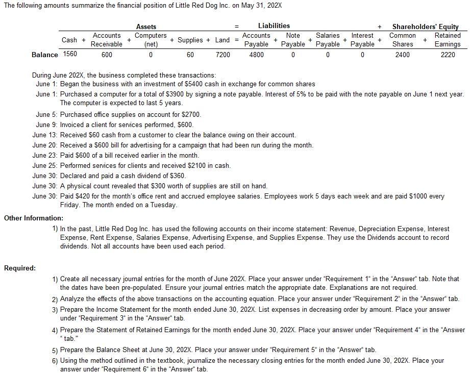
Build an Excel spreadsheet using the accounting equation (Assets = Liabilities + Shareholders' Equity). Remember that each transaction has an equal effect on both the left-hand side and the right-hand side of the equation or an offsetting effect (both positive and negative) on the same side of the equation.

1. Select the 'Answer' tab and locate 'Requirement 2'.

2) Format the worksheet. Label cell H4 "Trans". You will put transaction dates (1 — 30) corresponding to the transactions in the cells in column H. Row 3 will contain the elements of the accounting equation. Enter "Assets" in cell K3. Enter '= in cell N3 (note the " '" before the "=". This tells Excel to consider the equal sign text). Resize column N in order to match the size of the = sign by dragging the right edge of the column to the left. Enter "Liabilities + Shareholders' equity" in cell P3. Enter "Type of SE Transaction" (abbreviation for shareholders' equity) in cell U3. Now you will have a spreadsheet organized around the elements of the accounting equation: "Assets = Liabilities + Shareholders' equity" and, for all transactions impacting shareholders' equity, you will be able to enter the type (common shares, revenue, expenses, or dividends). This will be important for later when you construct the financial statements (Exhibit 2-2, page 65).

3) Continue formatting. In cells 14 through M4, enter the asset account titles that the transactions deal with. 14: Cash; J4: AR (an abbreviation for accounts receivable); K4: Computers & AD (an abbreviation for accumulated depreciation); L4: Supplies; M4: Land. In cells 04 through T4, enter the liability and shareholders' equity account titles that the company's transactions deal with. 04: AP (an abbreviation for accounts payable); P4: NP (an abbreviation for note payable); Q4: SP (an abbreviation for salaries payable); R4: IP (an abbreviation for interest payable); S4: Charles (an abbreviation for common shares); and T4: RE (abbreviation for retained earnings; this is where all transactions impacting revenue, expenses and dividends will go for now).

4) Before entering the transactions, sum each column from I through M and 0 through T in row 21. For example, the formula in cell 121 should be "=sum(15:120)", in cell J21 the formula should be "=sum(J5:J20)", and so on for each of the columns: I, J, K, L, M, 0, P, Q, R, S, and T. In cell H21, enter "Bal". This will allow you to keep a running sum of the accounts as you enter each transaction. For now, it will be a "0," but this will change as you enter the transactions.

5) In cell H22, enter "Totals". In cell 122, enter "=sum(I21:M21)." In cell 022, enter "=sum(021:T21)." Excel allows you to keep a running sum of the column totals on each side of the equation. You should find that the running sum of the column totals on the left-hand side of the equation always equals the running sum of the column totals on the right-hand side so the accounting equation is always in balance.

6) Highlight cells 15 through T22. On a PC, right-click on your selection and select "Format Cells". On a Mac, select "Format' then click "cells". Under the "number" tab, change the number format from "General" to "Accounting". In the same dialogue box, select the symbol dropdown menu and change "8" to "none' and reduce the number of decimal places to 0. Select "OK to close the dialogue box and save your settings.

7) As a final formatting step, highlight cells 14 to T4 and select the "bottom border' icon in the toolbar at the top of the spreadsheet (note that you might have to select this option using the small arrow beside the icon). Highlight Cells 121 to T21 and select the 'top border' icon from the same menu.

8) Enter the opening balances given in the problem in row 5.

9) Beginning in row 6, enter the transactions given in the problem. Use multiple rows as necessary.

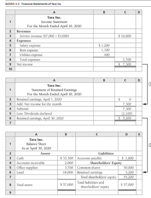
10) Using Exhibit 2-2 on page 65 as a guide, construct the financial statements for Requirements 3, 4, and 5. Place each requirement under its corresponding section under the "Answer" tab.

  
 

Transcribed Image Text:

Exhibit 2-2 Financial Statements of Tara Inc. 1 2 3 4 5 6 7 8 9 10 1 2 3 4 5 6 7 1 2 3 4 5 6 7 8 9 A Tara Inc. Income Statement For the Month Ended April 30, 2020 Revenues Service revenue ($7,000+ $3,000) Expenses Salary expense Rent expense Utilities expense Total expenses Net income A Tara Inc. Statement of Retained Earnings For the Month Ended April 30, 2020 Retained earnings, April 1, 2020 Add: Net income for the month Subtotal Less: Dividends declared Retained earnings, April 30, 2020 A Tara Inc. Balance Sheet As at April 30, 2020 Assets Cash Accounts receivable Office supplies Land Total assets B $33,300 2,000 3,700 18,000 $ 57,000 с B $1,200 1,100 400 Accounts payable B Liabilities Common shares Retained earnings Total shareholders' equity Total liabilities and shareholders' equity $10,000 с 2,700 $7,300 $ Shareholders' Equity с 0 7,300 7,300 (2,100) $ 5,200 D $ 1,800 50,000 5,200 55,200 $ 57,000 D D E Exhibit 2-2 Financial Statements of Tara Inc. 1 2 3 4 5 6 7 8 9 10 1 2 3 4 5 6 7 1 2 3 4 5 6 7 8 9 A Tara Inc. Income Statement For the Month Ended April 30, 2020 Revenues Service revenue ($7,000+ $3,000) Expenses Salary expense Rent expense Utilities expense Total expenses Net income A Tara Inc. Statement of Retained Earnings For the Month Ended April 30, 2020 Retained earnings, April 1, 2020 Add: Net income for the month Subtotal Less: Dividends declared Retained earnings, April 30, 2020 A Tara Inc. Balance Sheet As at April 30, 2020 Assets Cash Accounts receivable Office supplies Land Total assets B $33,300 2,000 3,700 18,000 $ 57,000 с B $1,200 1,100 400 Accounts payable B Liabilities Common shares Retained earnings Total shareholders' equity Total liabilities and shareholders' equity $10,000 с 2,700 $7,300 $ Shareholders' Equity с 0 7,300 7,300 (2,100) $ 5,200 D $ 1,800 50,000 5,200 55,200 $ 57,000 D D E