Answered step by step
Verified Expert Solution
Question
1 Approved Answer
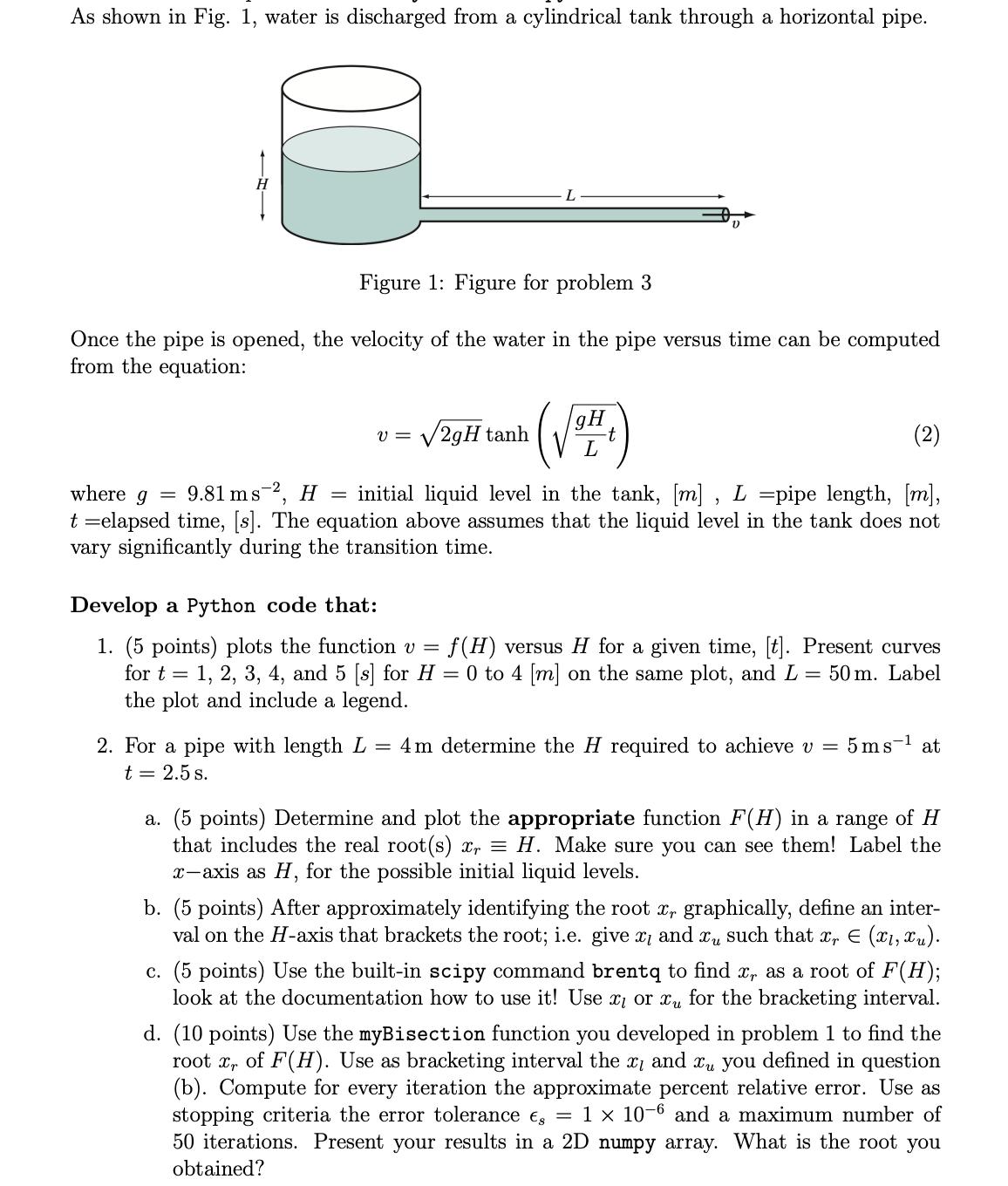
As shown in Fig. 1, water is discharged from a cylindrical tank through a horizontal pipe. Figure 1: Figure for problem 3 Once the


As shown in Fig. 1, water is discharged from a cylindrical tank through a horizontal pipe. Figure 1: Figure for problem 3 Once the pipe is opened, the velocity of the water in the pipe versus time can be computed from the equation: (2) where g = 9.81 ms 2, H = initial liquid level in the tank, [m], L =pipe length, [m], t =elapsed time, [s]. The equation above assumes that the liquid level in the tank does not vary significantly during the transition time. V2gH tanh V = V 9H L -t Develop a Python code that: 1. (5 points) plots the function v = f(H) versus H for a given time, [t]. Present curves for t= = 1, 2, 3, 4, and 5 [s] for H = 0 to 4 [m] on the same plot, and L = 50 m. Label the plot and include a legend. 2. For a pipe with length L = 4m determine the H required to achieve v = 5 ms at t = 2.5 s. a. (5 points) Determine and plot the appropriate function F(H) in a range of H that includes the real root(s) x = H. Make sure you can see them! Label the x-axis as H, for the possible initial liquid levels. b. (5 points) After approximately identifying the root x, graphically, define an inter- val on the H-axis that brackets the root; i.e. give x, and x, such that x, E (X1, Xu). c. (5 points) Use the built-in scipy command brentq to find x, as a root of F(H); look at the documentation how to use it! Use x or x for the bracketing interval. d. (10 points) Use the myBisection function you developed in problem 1 to find the root x of F(H). Use as bracketing interval the x, and xu you defined in question (b). Compute for every iteration the approximate percent relative error. Use as stopping criteria the error tolerance 1 x 10⁻⁶ and a maximum number of 50 iterations. Present your results in a 2D numpy array. What is the root you obtained? e. (10 points) Use the false myFalse Position function you developed in problem 2 to find the root xr of F(H). Use as bracketing interval the x and xu you defined in question (b). Compute for every iteration the approximate percent relative error. Use as stopping criteria the error tolerance = 1 10-6 and a maximum number of 50 iterations. Present your results in a 2D numpy array. What is the root you obtained? f. (5 points) Plot in a common figure (linear scale axes) the approximated root xr vs the number of iterations, for the solutions you obtained with the bisection and the false position methods in questions (d) and (e). g. (5 points) Plot in a common figure (semi-logarithmic on the y-axis, linear on the x-axis) the approximate relative percent error ea vs number of iterations, for the solutions you obtained with the bisection and the false position methods in questions (d) and (e). h. (10 points) Comment on the results and graphs of the previous questions. Which method performs better in this problem? Which method converges fastest to the exact solution? Make suggestions for improvement of the solutions if not satisfactory. As shown in Fig. 1, water is discharged from a cylindrical tank through a horizontal pipe. Figure 1: Figure for problem 3 Once the pipe is opened, the velocity of the water in the pipe versus time can be computed from the equation: (2) where g = 9.81 ms 2, H = initial liquid level in the tank, [m], L =pipe length, [m], t =elapsed time, [s]. The equation above assumes that the liquid level in the tank does not vary significantly during the transition time. V2gH tanh V = V 9H L -t Develop a Python code that: 1. (5 points) plots the function v = f(H) versus H for a given time, [t]. Present curves for t= = 1, 2, 3, 4, and 5 [s] for H = 0 to 4 [m] on the same plot, and L = 50 m. Label the plot and include a legend. 2. For a pipe with length L = 4m determine the H required to achieve v = 5 ms at t = 2.5 s. a. (5 points) Determine and plot the appropriate function F(H) in a range of H that includes the real root(s) x = H. Make sure you can see them! Label the x-axis as H, for the possible initial liquid levels. b. (5 points) After approximately identifying the root x, graphically, define an inter- val on the H-axis that brackets the root; i.e. give x, and x, such that x, E (X1, Xu). c. (5 points) Use the built-in scipy command brentq to find x, as a root of F(H); look at the documentation how to use it! Use x or x for the bracketing interval. d. (10 points) Use the myBisection function you developed in problem 1 to find the root x of F(H). Use as bracketing interval the x, and xu you defined in question (b). Compute for every iteration the approximate percent relative error. Use as stopping criteria the error tolerance 1 x 10⁻⁶ and a maximum number of 50 iterations. Present your results in a 2D numpy array. What is the root you obtained? e. (10 points) Use the false myFalse Position function you developed in problem 2 to find the root xr of F(H). Use as bracketing interval the x and xu you defined in question (b). Compute for every iteration the approximate percent relative error. Use as stopping criteria the error tolerance = 1 10-6 and a maximum number of 50 iterations. Present your results in a 2D numpy array. What is the root you obtained? f. (5 points) Plot in a common figure (linear scale axes) the approximated root xr vs the number of iterations, for the solutions you obtained with the bisection and the false position methods in questions (d) and (e). g. (5 points) Plot in a common figure (semi-logarithmic on the y-axis, linear on the x-axis) the approximate relative percent error ea vs number of iterations, for the solutions you obtained with the bisection and the false position methods in questions (d) and (e). h. (10 points) Comment on the results and graphs of the previous questions. Which method performs better in this problem? Which method converges fastest to the exact solution? Make suggestions for improvement of the solutions if not satisfactory. As shown in Fig. 1, water is discharged from a cylindrical tank through a horizontal pipe. Figure 1: Figure for problem 3 Once the pipe is opened, the velocity of the water in the pipe versus time can be computed from the equation: (2) where g = 9.81 ms 2, H = initial liquid level in the tank, [m], L =pipe length, [m], t =elapsed time, [s]. The equation above assumes that the liquid level in the tank does not vary significantly during the transition time. V2gH tanh V = V 9H L -t Develop a Python code that: 1. (5 points) plots the function v = f(H) versus H for a given time, [t]. Present curves for t= = 1, 2, 3, 4, and 5 [s] for H = 0 to 4 [m] on the same plot, and L= 50 m. Label the plot and include a legend. 2. For a pipe with length L = 4m determine the H required to achieve v = 5 ms at t = 2.5 s. a. (5 points) Determine and plot the appropriate function F(H) in a range of H that includes the real root(s) x = H. Make sure you can see them! Label the x-axis as H, for the possible initial liquid levels. b. (5 points) After approximately identifying the root x, graphically, define an inter- val on the H-axis that brackets the root; i.e. give x, and x, such that x, E (x1, xu). c. (5 points) Use the built-in scipy command brentq to find x, as a root of F(H); look at the documentation how to use it! Use x or x for the bracketing interval. d. (10 points) Use the myBisection function you developed in problem 1 to find the root x of F(H). Use as bracketing interval the x, and xu you defined in question (b). Compute for every iteration the approximate percent relative error. Use as stopping criteria the error tolerance 1 x 10⁻⁶ and a maximum number of 50 iterations. Present your results in a 2D numpy array. What is the root you obtained? e. (10 points) Use the false myFalsePosition function you developed in problem 2 to find the root xr of F(H). Use as bracketing interval the x and xu you defined in question (b). Compute for every iteration the approximate percent relative error. Use as stopping criteria the error tolerance = 1 10-6 and a maximum number of 50 iterations. Present your results in a 2D numpy array. What is the root you obtained? f. (5 points) Plot in a common figure (linear scale axes) the approximated root xr vs the number of iterations, for the solutions you obtained with the bisection and the false position methods in questions (d) and (e). g. (5 points) Plot in a common figure (semi-logarithmic on the y-axis, linear on the x-axis) the approximate relative percent error ea vs number of iterations, for the solutions you obtained with the bisection and the false position methods in questions (d) and (e). h. (10 points) Comment on the results and graphs of the previous questions. Which method performs better in this problem? Which method converges fastest to the exact solution? Make suggestions for improvement of the solutions if not satisfactory.
Step by Step Solution
★★★★★
3.30 Rating (162 Votes )
There are 3 Steps involved in it
Step: 1
import numpy as np import matplotlibpyplot as plt from scipyoptimize import brentq Constants g 981 ms2 L 500 Pipe length in meters epsilons 1e6 Error tolerance maxiterations 50 Maximum number of itera...
Get Instant Access to Expert-Tailored Solutions
See step-by-step solutions with expert insights and AI powered tools for academic success
Step: 2

Step: 3

Ace Your Homework with AI
Get the answers you need in no time with our AI-driven, step-by-step assistance
Get Started


