code: # -- coding: utf-8 -- Created on Fri Nov 27 18:27:23 2020 @author: willi

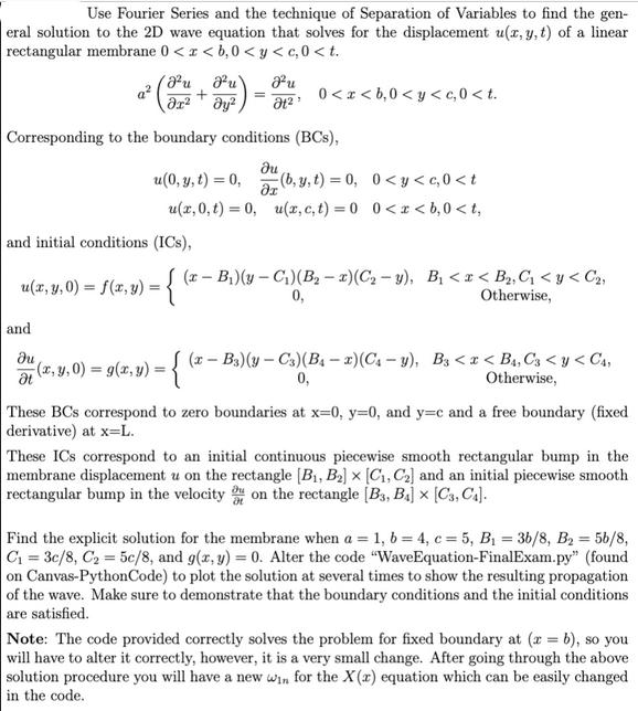
Fantastic news! We've Found the answer you've been seeking!

Question:

Use Fourier Series and the technique of Separation of Variables to find the gen- eral solution to the 2D wave

code:

# -*- coding: utf-8 -*-
"""
Created on Fri Nov 27 18:27:23 2020

@author: willi
"""

import numpy as np
import matplotlib.pyplot as plt
from matplotlib import cm

L1=4.0;L2=5.0;a=1.0;

# def f(x,y):
# return 1*(L1/4

# def A_mn(m,n,L1,L2):
# return (4/(L1*L2))*(2*L1*np.sin(m*np.pi/4)*np.sin(m*np.pi/2)/(np.pi*m))*(2*L2*np.sin(n*np.pi/4)*np.sin(n*np.pi/2)/(np.pi*n))

A1=3*L1/8
A2=5*L1/8

B1=3*L2/8
B2=5*L2/8

def f(x,y):
return (x-A1)*(y-B1)*(A2-x)*(B2-y)*(A1 M=f(L1/2,L2/2);

######
## The following function definition for w_1m
## is the only change you have to make for the final exam problem
def w_1m(m):
return m*np.pi/L1

## everything else (initial conditions, etc.) is set up correctly
## for the final problem.

def w_2n(n):
return n*np.pi/L2

def w_mn(m,n):
return np.sqrt( w_1m(m)**2+w_2n(n)**2 )

def A_mn(m,n):
S1=(np.sin(w_1m(m)*A1)+np.sin(w_1m(m)*A2))
C1=(np.cos(w_1m(m)*A1)-np.cos(w_1m(m)*A2))

S2=(np.sin(w_2n(n)*B1)+np.sin(w_2n(n)*B2))
C2=(np.cos(w_2n(n)*B1)-np.cos(w_2n(n)*B2))

A1m=(1/(w_1m(m))**3)*(w_1m(m)*(A1-A2)*S1+2*C1)
A2n=(1/(w_2n(n))**3)*(w_2n(n)*(B1-B2)*S2+2*C2)
return (4/(L1*L2))*A1m*A2n

def B_mn(m,n):
return 0

# a_list=np.array([an(i,P) for i in n_list])
N_l=100

n_list=np.arange(N_l)+1
m_list=np.arange(N_l)+1

# return np.sum(uu,axis=0)

nn=100

x_pl=np.linspace(0,L1,nn)
y_pl=np.linspace(0,L2,nn)

X,Y=np.meshgrid(x_pl,y_pl)

def u(x,y,t,N=N_l,M=N_l):
uu=np.array([A_mn(m,n)*np.cos(w_mn(m,n)*a*t)*np.sin(w_1m(m)*x)*np.sin(w_2n(n)*y)+B_mn(m,n)*np.sin(w_mn(m,n)*a*t)*np.sin(w_1m(m)*x)*np.sin(w_2n(n)*y) for n in np.arange(N)+1 for m in np.arange(M)+1])
return np.sum(uu,axis=0)

pl_M=M/3

t_S=2.0;

tS_R=np.round(t_S,3)

fig = plt.figure('Wave Equation')
plt.clf()

ax = plt.subplot(121,projection='3d')

ax.plot_surface(X,Y,f(X,Y),alpha=0.7)

ax.plot_surface(X,Y,u(X,Y,t_S),vmin=-pl_M,vmax=pl_M,cmap=cm.coolwarm,alpha=.9)

ax.view_init(elev=20., azim=-40)

(ax.set_title('Truncated FS Solution to '+' Linear 2D Wave Equation '+
r'$a^2\left(\frac{\partial^2 u}{\partial x^2}+\frac{\partial^2 u}{\partial y^2}ight)=\frac{\partial^2 u}{\partial t^2}$, '+'a='+str(np.round(a,3))+''+
r'$u(x,y,t)$ at $t=$'+str(tS_R),fontsize=12))

# ax.plot(x_pl,u(x_pl,0.1))

ax.set_xlim([0,L1])
ax.set_ylim([0,L2])
ax.set_zlim([-M,M])

ax.set_xlabel('x')
ax.set_ylabel('y')
ax.view_init(elev=20., azim=-40)

# ax.set_zlabel('Wave Height')

ax3=plt.subplot(1,2,2)

# waveh=ax3.pcolormesh(X_pl,Y_pl,f(X_pl,Y_pl),vmin=-pl_M,vmax=pl_M, cmap=cm.coolwarm)

waveh=ax3.pcolormesh(X,Y,u(X,Y,t_S),shading='nearest',vmin=-pl_M,vmax=pl_M, cmap=cm.coolwarm)

plt.colorbar(waveh)

ax3.set_xlim([0,L1])
ax3.set_ylim([0,L2])

plt.axis('equal')

fig.tight_layout(h_pad=10)

plt.show()

# # Animation Image Production Code

# frames=1000;
# T_0=0.0;T_f=10.0;

# tt=np.linspace(T_0,T_f,frames);
# tt_R=np.round(tt,3)

# fig2 = plt.figure('Wave Equation Animation')

# for i in np.arange(tt.size):
# plt.clf()
# plt.cla()

# ax2 = plt.subplot(121,projection='3d')

# ax2.plot_surface(X,Y,f(X,Y),alpha=0.5)

# ax2.plot_surface(X,Y,u(X,Y,tt[i]),vmin=-pl_M,vmax=pl_M,alpha=.9,cmap=cm.coolwarm)

# ax2.view_init(elev=20., azim=-40)

# # ax.plot(x_pl,u(x_pl,0.1))

# ax2.set_xlim([0,L1])
# ax2.set_ylim([0,L2])
# ax2.set_zlim([-M,M])

# ax2.set_xlabel('x')
# ax2.set_ylabel('y')
# ax2.view_init(elev=20., azim=-40)

# (ax2.set_title('Truncated FS Solution to '+' Linear 2D Wave Equation '+
# r'$a^2\left(\frac{\partial^2 u}{\partial x^2}+\frac{\partial^2 u}{\partial y^2}ight)=\frac{\partial^2 u}{\partial t^2}$, '+'a='+str(np.round(a,3))+''+
# r'$u(x,y,t)$ at $t=$'+str(tt_R[i]),fontsize=12))

# # ax2.set_zlabel('Wave Height')

# ax4=plt.subplot(1,2,2)
# waveh=ax4.pcolormesh(X,Y,u(X,Y,tt[i]),shading='nearest',vmin=-pl_M,vmax=pl_M,cmap=cm.coolwarm)

# plt.colorbar(waveh)

# # ax4.set_xlabel('x')
# # ax4.set_ylabel('y')

# ax4.set_xlim([0,L1])
# ax4.set_ylim([0,L2])

# plt.axis('equal')

# fig2.tight_layout(h_pad=10)