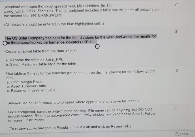
Download and open the excel spreadsheet, Miller-Nobles_6e-12e- Using Excel_Ch24_Start.xlsx. This spreadsheet includes 2 tabs; you will...

 

  
 
 
 
 
 

Transcribed Image Text:

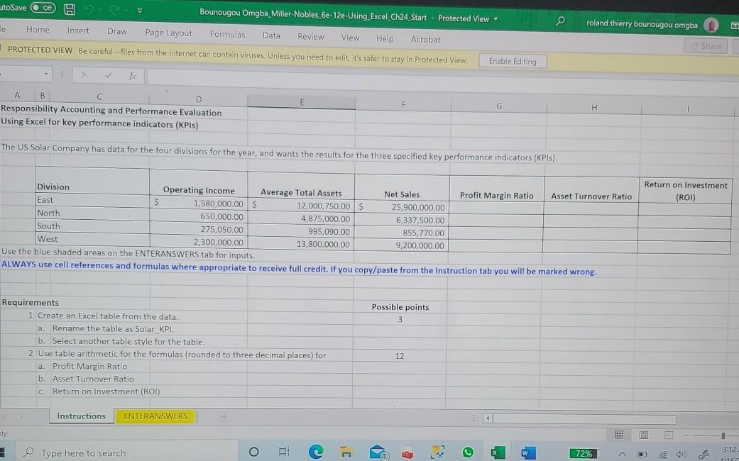
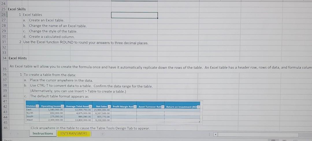
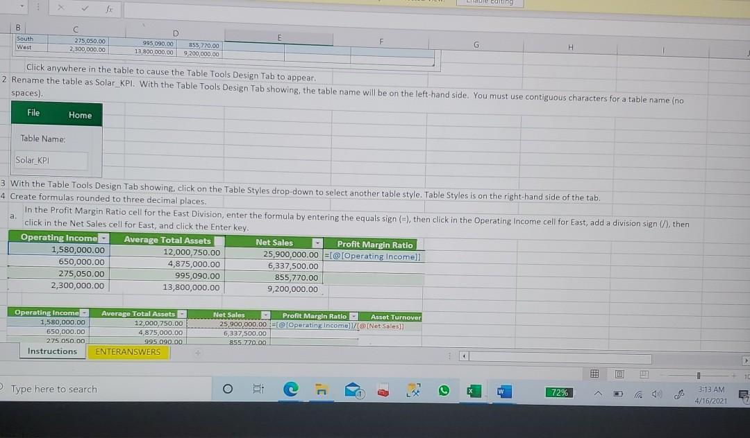
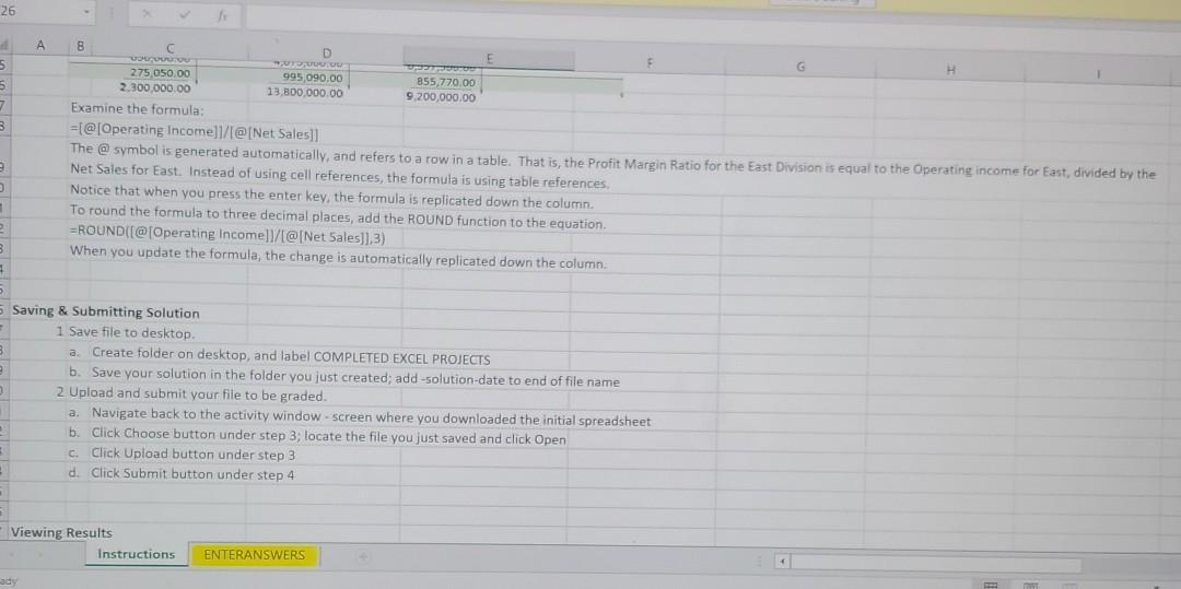
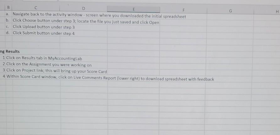
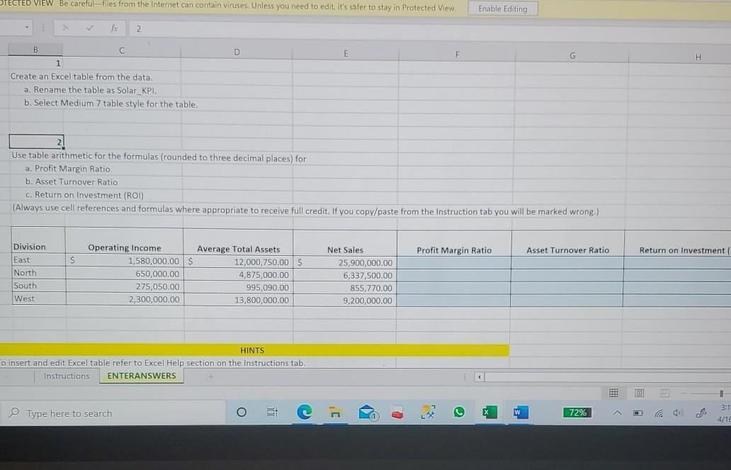
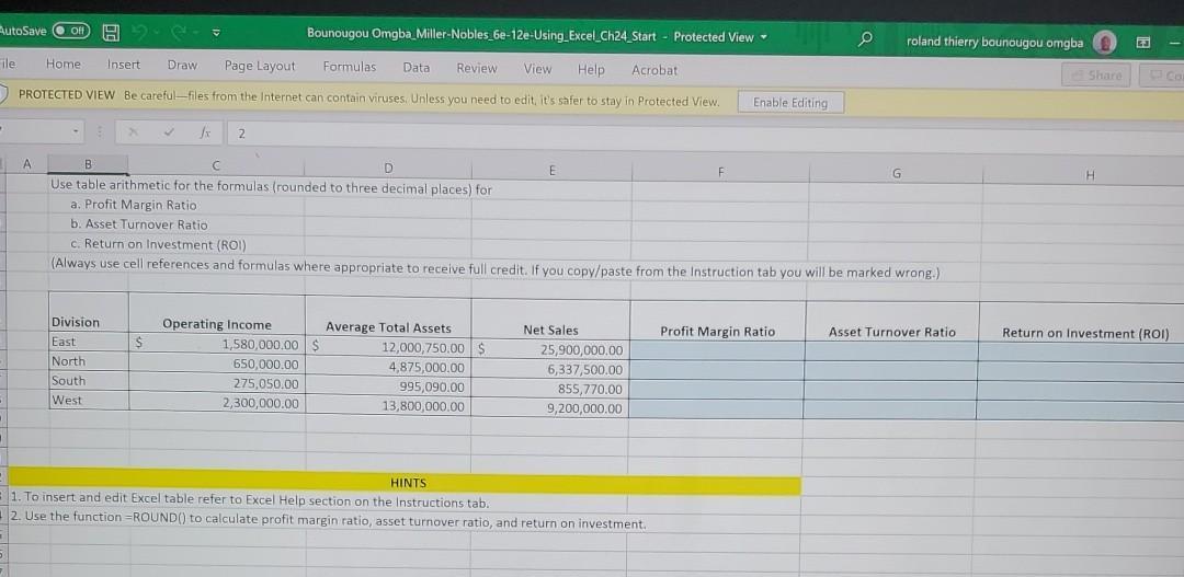
Download and open the excel spreadsheet, Miller-Nobles_6e-12e- Using Excel_Ch24_Start.xlsx. This spreadsheet includes 2 tabs; you will enter all answers on the second tab, ENTERANSWERS. (All answers should be entered in the blue highlighted cells.) The US Solar Company has data for the four divisions for the year, and wants the results for Oe three specified key performance indicators (KPIs). O Create an Excel table from the data. (3 pts) a. Rename the table as Solar_KPI. b. Select Medium 7 table style for the table. Use table arithmetic for the formulas (rounded to three decimal places) for the following: (12 pts) a. Profit Margin Ratio b. Asset Turnover Ratio c. Return on Investment (ROI) (Always use cell references and formulas where appropriate to receive full credit.) Once completed, save the project to the desktop. File name can be anything, but DO NOT include spaces. Return to auto-graded excel activity window, and progress to Step 3. Follow on screen instructions. (To review score, navigate to Results in the MyLab and click on Review link.) 0 3 12 D Focus utoSave Off H le Bounougou Omgba_Miller-Nobles_6e-12e-Using Excel_Ch24_Start Protected View Insert Draw Page Layout Formulas Data: Review View Help. Acrobat PROTECTED VIEW Be careful-files from the Internet can contain viruses. Unless you need to edit, it's safer to stay in Protected View. Home ly 3 Requirements A B Responsibility Accounting and Performance Evaluation Using Excel for key performance indicators (KPIs) The US Solar Company has data for the four divisions for the year, and wants the results for the three specified key performance indicators (KPIs). a. Profit Margin Ratio b. Asset Turnover Ratio C. S 1 Create an Excel table from the data. a. Rename the table as Solar_KPI.. b. Select another table style for the table. 2 Use table arithmetic for the formulas (rounded to three decimal places) for Return on Investment (ROI) Instructions ENTERANSWERS Type here to search Division East Operating Income: Average Total Assets 1,580,000.00 $ 650,000.00 North South 275,050.00 West 2,300,000.00 Use the blue shaded areas on the ENTERANSWERS tab for inputs. ALWAYS use cell references and formulas where appropriate to receive full credit. If you copy/paste from the Instruction tab you will be marked wrong. E O | 12,000,750.00 $ 4,875,000.00 995,090.00 13,800,000.00 3¹ F O - Possible points 3 Net Sales 25,900,000.00 6,337,500.00 855,770.00 9.200,000.00 12 Enable Editing F* G 0 A roland thierry bounougou omgba W Profit Margin Ratio Asset Turnover Ratio H 72% Return on Investment (ROI) E ^ E Share Co 4 Js 1 53 3:12 11150 24 25 Excel Skills 26 27 28 29 30 31 32 33 34 Excel Hints 1 Excel tables a. Create an Excel table. b. Change the name of an Excel table. c. Change the style of the table. d. Create a calculated column. 2 Use the Excel function ROUND to round your answers to three decimal places. An Excel table will allow you to create the formula once and have it automatically replicate down the rows of the table. An Excel table has a header row, rows of data, and formula colum 35 36 1 To create a table from the data: 37 a. Place the cursor anywhere in the data. 38 b. Use CTRL-T to convert data to a table. Confirm the data range for the table. 39 (Alternatively, you can use Insert > Table to create a table.) 40 c. The default table format appears as 41 42 43 44 45 46 Readi Division Operating Incom Average Total Asset 1,580,000.00 650,000.00 275,050.00 2,300,000.00 East North South West Net Sales Profit Margin Rati Asset Turnover Rati- Return on investment (RO 25,900,000.00 12,000,750.00 4,875,000.00 6,337,500.00 995,090.00 855,770.00 13,800,000.00 9,200,000.00 Click anywhere in the table to cause the Table Tools Design Tab to appear. Instructions ENTERANSWERS 4 C F B South West Table Name: Solar KPI C a. 275,050.00 2,300,000.00 Home Click anywhere in the table to cause the Table Tools Design Tab to appear. 2 Rename the table as Solar_KPI. With the Table Tools Design Tab showing, the table name will be on the left-hand side. You must use contiguous characters for a table name (no spaces). File fix Operating Income- 1,580,000.00 650,000.00 275,050.00 2,300,000.00 Operating Income 1,580,000.00 650,000.00 275.050.00 3 With the Table Tools Design Tab showing, click on the Table Styles drop-down to select another table style. Table Styles is on the right-hand side of the tab. 4 Create formulas rounded to three decimal places. Instructions D 995,090,00 855,770.00 13,800,000.00 9,200,000.00 In the Profit Margin Ratio cell for the East Division, enter the formula by entering the equals sign (=), then click in the Operating Income cell for East, add a division sign (/), then click in the Net Sales cell for East, and click the Enter key. Average Total Assets Type here to search ENTERANSWERS E 12,000,750.00 4,875,000.00 995,090.00 13,800,000.00 Average Total Assets- 12,000,750.00 4,875,000.00 995.090.00 F Net Sales Profit Margin Ratio 25,900,000.00 =[@[Operating Income]] 6,337,500.00 Et 855,770.00 9,200,000.00 H Net Sales Profit Margin Ratio Asset Turnover 25,900,000.00 [@[Operating Income]]/[@[Net Sales]] 6,337,500.00 855.770.00 < 72% ^ 3:13 AM 4/16/2021 > +11 10 E 26 4 7 3 3 0.1 1 2 B 9 0 3 5 Saving & Submitting Solution 1 Save file to desktop. E A 11 B C 200.00 275,050.00 2,300,000.00 Examine the formula: =[@[Operating Income]]/[@[Net Sales]] The @symbol is generated automatically, and refers to a row in a table. That is, the Profit Margin Ratio for the East Division is equal to the Operating income for East, divided by the Net Sales for East. Instead of using cell references, the formula is using table references. Notice that when you press the enter key, the formula is replicated down the column. To round the formula to three decimal places, add the ROUND function to the equation. =ROUND([@[Operating Income]]/[@[Net Sales]],3) When you update the formula, the change is automatically replicated down the column. Viewing Results D 070,000,00 995,090.00 13,800,000.00 a. Create folder on desktop, and label COMPLETED EXCEL PROJECTS b. Save your solution in the folder you just created; add-solution-date to end of file name 2 Upload and submit your file to be graded. a. Navigate back to the activity window - screen where you downloaded the initial spreadsheet b. Click Choose button under step 3; locate the file you just saved and click Open c. Click Upload button under step 3 d. Click Submit button under step 4 Instructions 855,770.00 9,200,000.00 ENTERANSWERS B E a. Navigate back to the activity window - screen where you downloaded the initial spreadsheet b. Click Choose button under step 3; locate the file you just saved and click Open c. Click Upload button under step 3 d. Click Submit button under step 4 ng Results 1 Click on Results tab in MyAccountingLab 2 Click on the Assignment you were working on 3 Click on Project link; this will bring up your Score Card 4 Within Score Card window, click on Live Comments Report (lower right) to download spreadsheet with feedback H OTECTED VIEW Be careful files from the Internet can contain viruses. Unless you need to edit, it's safer to stay in Protected View. B 1 Create an Excel table from the data. a. Rename the table as Solar_KPI. b. Select Medium 7 table style for the table. C Division East North South West 2 2 Use table arithmetic for the formulas (rounded to three decimal places) for a. Profit Margin Ratio, b. Asset Turnover Ratio: $ Operating Income. Type here to search D c. Return on Investment (ROI) (Always use cell references and formulas where appropriate to receive full credit. If you copy/paste from the Instruction tab you will be marked wrong.) 1,580,000.00 $ 650,000.00 275,050.00 2,300,000.00 Average Total Assets 12,000,750.00 $ 4,875,000.00 995,090.00 13,800,000.00 HINTS o insert and edit Excel table refer to Excel Help section on the Instructions tab. Instructions: ENTERANSWERS O Et E Net Sales 25,900,000,00 6,337,500.00 855,770.00 9,200,000.00 C D Enable Editing KA Profit Margin Ratio G W Asset Turnover Ratio. 72% ^ H Return on Investment ( 4 J 1 3:1 4/16 AutoSave Off HC- Bounougou Omgba_Miller-Nobles_6e-12e-Using Excel_Ch24_Start Protected View File Home Insert Draw Page Layout Formulas Data Review View Help Acrobat PROTECTED VIEW Be careful-files from the Internet can contain viruses. Unless you need to edit, it's safer to stay in Protected View. D A Jx B C D Use table arithmetic for the formulas (rounded to three decimal places) for a. Profit Margin Ration b. Asset Turnover Ratio: Division East North South West 2 $ Operating Income 1,580,000.00 $ 650,000.00 275,050.00 2,300,000.00 Average Total Assets c. Return on Investment (ROI) (Always use cell references and formulas where appropriate to receive full credit. If you copy/paste from the Instruction tab you will be marked wrong.) 12,000,750.00 $ 4,875,000.00 995,090.00 13,800,000.00 E HINTS Net Sales 25,900,000.00 6,337,500.00 855,770.00 9,200,000.00 F 1. To insert and edit Excel table refer to Excel Help section on the Instructions tab. 2. Use the function=ROUND() to calculate profit margin ratio, asset turnover ratio, and return on investment. Enable Editing G Profit Margin Ratio roland thierry bounougou omgba Asset Turnover Ratio 23 Share Co H Return on Investment (ROI) Download and open the excel spreadsheet, Miller-Nobles_6e-12e- Using Excel_Ch24_Start.xlsx. This spreadsheet includes 2 tabs; you will enter all answers on the second tab, ENTERANSWERS. (All answers should be entered in the blue highlighted cells.) The US Solar Company has data for the four divisions for the year, and wants the results for Oe three specified key performance indicators (KPIs). O Create an Excel table from the data. (3 pts) a. Rename the table as Solar_KPI. b. Select Medium 7 table style for the table. Use table arithmetic for the formulas (rounded to three decimal places) for the following: (12 pts) a. Profit Margin Ratio b. Asset Turnover Ratio c. Return on Investment (ROI) (Always use cell references and formulas where appropriate to receive full credit.) Once completed, save the project to the desktop. File name can be anything, but DO NOT include spaces. Return to auto-graded excel activity window, and progress to Step 3. Follow on screen instructions. (To review score, navigate to Results in the MyLab and click on Review link.) 0 3 12 D Focus utoSave Off H le Bounougou Omgba_Miller-Nobles_6e-12e-Using Excel_Ch24_Start Protected View Insert Draw Page Layout Formulas Data: Review View Help. Acrobat PROTECTED VIEW Be careful-files from the Internet can contain viruses. Unless you need to edit, it's safer to stay in Protected View. Home ly 3 Requirements A B Responsibility Accounting and Performance Evaluation Using Excel for key performance indicators (KPIs) The US Solar Company has data for the four divisions for the year, and wants the results for the three specified key performance indicators (KPIs). a. Profit Margin Ratio b. Asset Turnover Ratio C. S 1 Create an Excel table from the data. a. Rename the table as Solar_KPI.. b. Select another table style for the table. 2 Use table arithmetic for the formulas (rounded to three decimal places) for Return on Investment (ROI) Instructions ENTERANSWERS Type here to search Division East Operating Income: Average Total Assets 1,580,000.00 $ 650,000.00 North South 275,050.00 West 2,300,000.00 Use the blue shaded areas on the ENTERANSWERS tab for inputs. ALWAYS use cell references and formulas where appropriate to receive full credit. If you copy/paste from the Instruction tab you will be marked wrong. E O | 12,000,750.00 $ 4,875,000.00 995,090.00 13,800,000.00 3¹ F O - Possible points 3 Net Sales 25,900,000.00 6,337,500.00 855,770.00 9.200,000.00 12 Enable Editing F* G 0 A roland thierry bounougou omgba W Profit Margin Ratio Asset Turnover Ratio H 72% Return on Investment (ROI) E ^ E Share Co 4 Js 1 53 3:12 11150 24 25 Excel Skills 26 27 28 29 30 31 32 33 34 Excel Hints 1 Excel tables a. Create an Excel table. b. Change the name of an Excel table. c. Change the style of the table. d. Create a calculated column. 2 Use the Excel function ROUND to round your answers to three decimal places. An Excel table will allow you to create the formula once and have it automatically replicate down the rows of the table. An Excel table has a header row, rows of data, and formula colum 35 36 1 To create a table from the data: 37 a. Place the cursor anywhere in the data. 38 b. Use CTRL-T to convert data to a table. Confirm the data range for the table. 39 (Alternatively, you can use Insert > Table to create a table.) 40 c. The default table format appears as 41 42 43 44 45 46 Readi Division Operating Incom Average Total Asset 1,580,000.00 650,000.00 275,050.00 2,300,000.00 East North South West Net Sales Profit Margin Rati Asset Turnover Rati- Return on investment (RO 25,900,000.00 12,000,750.00 4,875,000.00 6,337,500.00 995,090.00 855,770.00 13,800,000.00 9,200,000.00 Click anywhere in the table to cause the Table Tools Design Tab to appear. Instructions ENTERANSWERS 4 C F B South West Table Name: Solar KPI C a. 275,050.00 2,300,000.00 Home Click anywhere in the table to cause the Table Tools Design Tab to appear. 2 Rename the table as Solar_KPI. With the Table Tools Design Tab showing, the table name will be on the left-hand side. You must use contiguous characters for a table name (no spaces). File fix Operating Income- 1,580,000.00 650,000.00 275,050.00 2,300,000.00 Operating Income 1,580,000.00 650,000.00 275.050.00 3 With the Table Tools Design Tab showing, click on the Table Styles drop-down to select another table style. Table Styles is on the right-hand side of the tab. 4 Create formulas rounded to three decimal places. Instructions D 995,090,00 855,770.00 13,800,000.00 9,200,000.00 In the Profit Margin Ratio cell for the East Division, enter the formula by entering the equals sign (=), then click in the Operating Income cell for East, add a division sign (/), then click in the Net Sales cell for East, and click the Enter key. Average Total Assets Type here to search ENTERANSWERS E 12,000,750.00 4,875,000.00 995,090.00 13,800,000.00 Average Total Assets- 12,000,750.00 4,875,000.00 995.090.00 F Net Sales Profit Margin Ratio 25,900,000.00 =[@[Operating Income]] 6,337,500.00 Et 855,770.00 9,200,000.00 H Net Sales Profit Margin Ratio Asset Turnover 25,900,000.00 [@[Operating Income]]/[@[Net Sales]] 6,337,500.00 855.770.00 < 72% ^ 3:13 AM 4/16/2021 > +11 10 E 26 4 7 3 3 0.1 1 2 B 9 0 3 5 Saving & Submitting Solution 1 Save file to desktop. E A 11 B C 200.00 275,050.00 2,300,000.00 Examine the formula: =[@[Operating Income]]/[@[Net Sales]] The @symbol is generated automatically, and refers to a row in a table. That is, the Profit Margin Ratio for the East Division is equal to the Operating income for East, divided by the Net Sales for East. Instead of using cell references, the formula is using table references. Notice that when you press the enter key, the formula is replicated down the column. To round the formula to three decimal places, add the ROUND function to the equation. =ROUND([@[Operating Income]]/[@[Net Sales]],3) When you update the formula, the change is automatically replicated down the column. Viewing Results D 070,000,00 995,090.00 13,800,000.00 a. Create folder on desktop, and label COMPLETED EXCEL PROJECTS b. Save your solution in the folder you just created; add-solution-date to end of file name 2 Upload and submit your file to be graded. a. Navigate back to the activity window - screen where you downloaded the initial spreadsheet b. Click Choose button under step 3; locate the file you just saved and click Open c. Click Upload button under step 3 d. Click Submit button under step 4 Instructions 855,770.00 9,200,000.00 ENTERANSWERS B E a. Navigate back to the activity window - screen where you downloaded the initial spreadsheet b. Click Choose button under step 3; locate the file you just saved and click Open c. Click Upload button under step 3 d. Click Submit button under step 4 ng Results 1 Click on Results tab in MyAccountingLab 2 Click on the Assignment you were working on 3 Click on Project link; this will bring up your Score Card 4 Within Score Card window, click on Live Comments Report (lower right) to download spreadsheet with feedback H OTECTED VIEW Be careful files from the Internet can contain viruses. Unless you need to edit, it's safer to stay in Protected View. B 1 Create an Excel table from the data. a. Rename the table as Solar_KPI. b. Select Medium 7 table style for the table. C Division East North South West 2 2 Use table arithmetic for the formulas (rounded to three decimal places) for a. Profit Margin Ratio, b. Asset Turnover Ratio: $ Operating Income. Type here to search D c. Return on Investment (ROI) (Always use cell references and formulas where appropriate to receive full credit. If you copy/paste from the Instruction tab you will be marked wrong.) 1,580,000.00 $ 650,000.00 275,050.00 2,300,000.00 Average Total Assets 12,000,750.00 $ 4,875,000.00 995,090.00 13,800,000.00 HINTS o insert and edit Excel table refer to Excel Help section on the Instructions tab. Instructions: ENTERANSWERS O Et E Net Sales 25,900,000,00 6,337,500.00 855,770.00 9,200,000.00 C D Enable Editing KA Profit Margin Ratio G W Asset Turnover Ratio. 72% ^ H Return on Investment ( 4 J 1 3:1 4/16 AutoSave Off HC- Bounougou Omgba_Miller-Nobles_6e-12e-Using Excel_Ch24_Start Protected View File Home Insert Draw Page Layout Formulas Data Review View Help Acrobat PROTECTED VIEW Be careful-files from the Internet can contain viruses. Unless you need to edit, it's safer to stay in Protected View. D A Jx B C D Use table arithmetic for the formulas (rounded to three decimal places) for a. Profit Margin Ration b. Asset Turnover Ratio: Division East North South West 2 $ Operating Income 1,580,000.00 $ 650,000.00 275,050.00 2,300,000.00 Average Total Assets c. Return on Investment (ROI) (Always use cell references and formulas where appropriate to receive full credit. If you copy/paste from the Instruction tab you will be marked wrong.) 12,000,750.00 $ 4,875,000.00 995,090.00 13,800,000.00 E HINTS Net Sales 25,900,000.00 6,337,500.00 855,770.00 9,200,000.00 F 1. To insert and edit Excel table refer to Excel Help section on the Instructions tab. 2. Use the function=ROUND() to calculate profit margin ratio, asset turnover ratio, and return on investment. Enable Editing G Profit Margin Ratio roland thierry bounougou omgba Asset Turnover Ratio 23 Share Co H Return on Investment (ROI)