the sensitivity of the slope of the AD curve to assumptions about how fiscal policy is...

 

  

Transcribed Image Text:

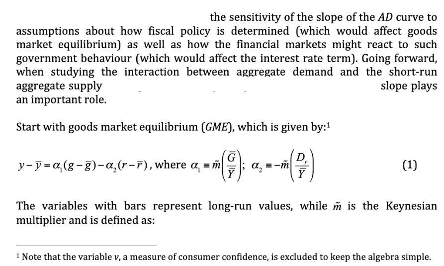
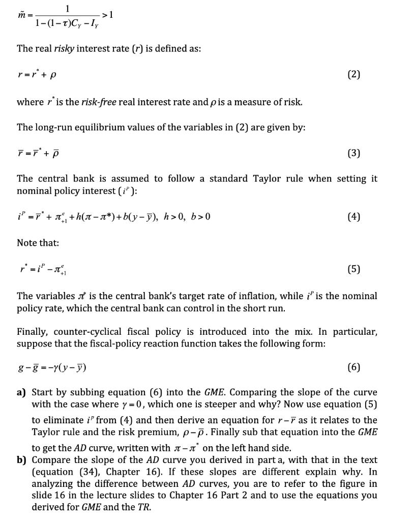
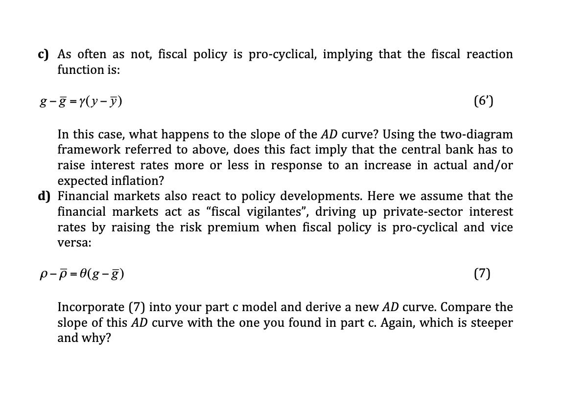
the sensitivity of the slope of the AD curve to assumptions about how fiscal policy is determined (which would affect goods market equilibrium) as well as how the financial markets might react to such government behaviour (which would affect the interest rate term). Going forward, when studying the interaction between aggregate demand and the short-run aggregate supply slope plays an important role. Start with goods market equilibrium (GME), which is given by:¹ - (2) Y G y-y=a (g-g) - a₂ (r-r), where a₁ = m * (*): Y a₂ = -m (1) The variables with bars represent long-run values, while m is the Keynesian multiplier and is defined as: 1 Note that the variable v, a measure of consumer confidence, is excluded to keep the algebra simple. 1 1-(1-T)Cy - Iy The real risky interest rate (r) is defined as: m = r=r + p ->1 Note that: (2) where r' is the risk-free real interest rate and p is a measure of risk. The long-run equilibrium values of the variables in (2) are given by: T=F¹ + P (3) The central bank is assumed to follow a standard Taylor rule when setting it nominal policy interest (i): i² = ¹ +²₁₁ +h(л−л*)+b(y-ỹ), h>0, b>0 (4) (5) The variables is the central bank's target rate of inflation, while i' is the nominal policy rate, which the central bank can control in the short run. Finally, counter-cyclical fiscal policy is introduced into the mix. In particular, suppose that the fiscal-policy reaction function takes the following form: g-g=-y(y-y) (6) a) Start by subbing equation (6) into the GME. Comparing the slope of the curve with the case where y = 0, which one is steeper and why? Now use equation (5) to eliminate i" from (4) and then derive an equation for r- as it relates to the Taylor rule and the risk premium, p-p. Finally sub that equation into the GME to get the AD curve, written with л-л on the left hand side. b) Compare the slope of the AD curve you derived in part a, with that in the text (equation (34), Chapter 16). If these slopes are different explain why. In analyzing the difference between AD curves, you are to refer to the figure in slide 16 in the lecture slides to Chapter 16 Part 2 and to use the equations you derived for GME and the TR. c) As often as not, fiscal policy is pro-cyclical, implying that the fiscal reaction function is: g-g=y(y-y) (6') In this case, what happens to the slope of the AD curve? Using the two-diagram framework referred to above, does this fact imply that the central bank has to raise interest rates more or less in response to an increase in actual and/or expected inflation? d) Financial markets also react to policy developments. Here we assume that the financial markets act as "fiscal vigilantes", driving up private-sector interest rates by raising the risk premium when fiscal policy is pro-cyclical and vice versa: p-p=0(g-g) Incorporate (7) into your part c model and derive a new AD curve. Compare the slope of this AD curve with the one you found in part c. Again, which is steeper and why? (7) the sensitivity of the slope of the AD curve to assumptions about how fiscal policy is determined (which would affect goods market equilibrium) as well as how the financial markets might react to such government behaviour (which would affect the interest rate term). Going forward, when studying the interaction between aggregate demand and the short-run aggregate supply slope plays an important role. Start with goods market equilibrium (GME), which is given by:¹ - (2) Y G y-y=a (g-g) - a₂ (r-r), where a₁ = m * (*): Y a₂ = -m (1) The variables with bars represent long-run values, while m is the Keynesian multiplier and is defined as: 1 Note that the variable v, a measure of consumer confidence, is excluded to keep the algebra simple. 1 1-(1-T)Cy - Iy The real risky interest rate (r) is defined as: m = r=r + p ->1 Note that: (2) where r' is the risk-free real interest rate and p is a measure of risk. The long-run equilibrium values of the variables in (2) are given by: T=F¹ + P (3) The central bank is assumed to follow a standard Taylor rule when setting it nominal policy interest (i): i² = ¹ +²₁₁ +h(л−л*)+b(y-ỹ), h>0, b>0 (4) (5) The variables is the central bank's target rate of inflation, while i' is the nominal policy rate, which the central bank can control in the short run. Finally, counter-cyclical fiscal policy is introduced into the mix. In particular, suppose that the fiscal-policy reaction function takes the following form: g-g=-y(y-y) (6) a) Start by subbing equation (6) into the GME. Comparing the slope of the curve with the case where y = 0, which one is steeper and why? Now use equation (5) to eliminate i" from (4) and then derive an equation for r- as it relates to the Taylor rule and the risk premium, p-p. Finally sub that equation into the GME to get the AD curve, written with л-л on the left hand side. b) Compare the slope of the AD curve you derived in part a, with that in the text (equation (34), Chapter 16). If these slopes are different explain why. In analyzing the difference between AD curves, you are to refer to the figure in slide 16 in the lecture slides to Chapter 16 Part 2 and to use the equations you derived for GME and the TR. c) As often as not, fiscal policy is pro-cyclical, implying that the fiscal reaction function is: g-g=y(y-y) (6') In this case, what happens to the slope of the AD curve? Using the two-diagram framework referred to above, does this fact imply that the central bank has to raise interest rates more or less in response to an increase in actual and/or expected inflation? d) Financial markets also react to policy developments. Here we assume that the financial markets act as "fiscal vigilantes", driving up private-sector interest rates by raising the risk premium when fiscal policy is pro-cyclical and vice versa: p-p=0(g-g) Incorporate (7) into your part c model and derive a new AD curve. Compare the slope of this AD curve with the one you found in part c. Again, which is steeper and why? (7)