• 
  

  

  

  
  

  Extend Example 2.2 (PV Model under Uncertainty) by doing the "2nd Year":

  -Assume 1st Year was a BAD Year ex-post

  -Assume 1st Year was a GOOD year ex-post.

Transcribed Image Text:

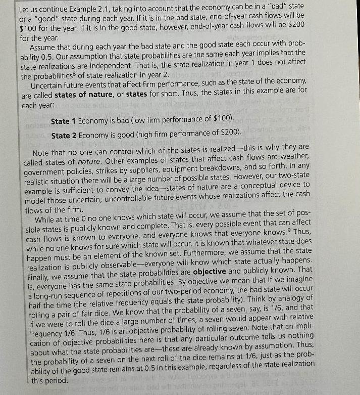
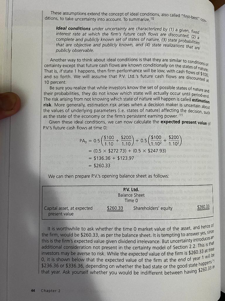
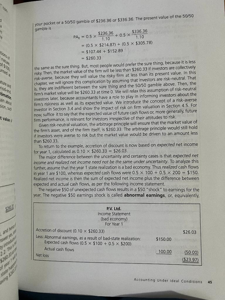
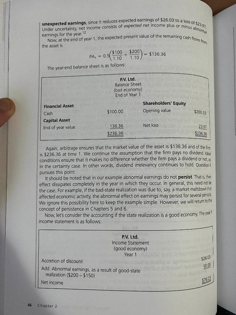
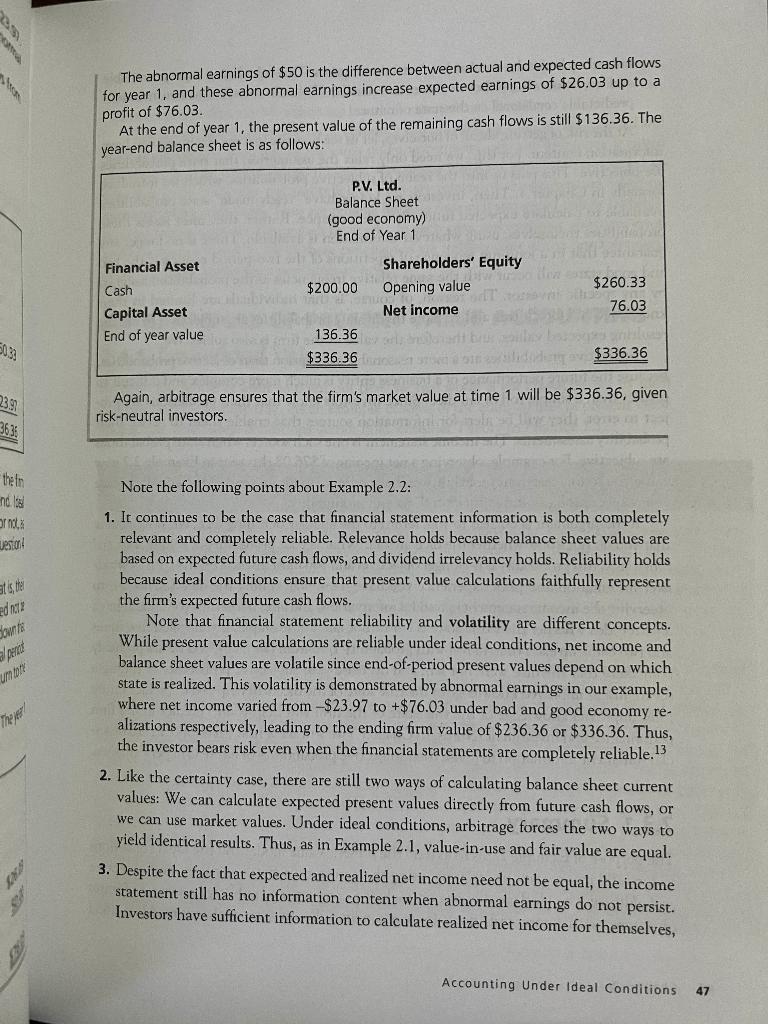
Let us continue Example 2.1, taking into account that the economy can be in a bad state or a good state during each year. If it is in the bad state, end-of-year cash flows will be $100 for the year. If it is in the good state, however, end-of-year cash flows will be $200 for the year. Assume that during each year the bad state and the good state each occur with prob- ability 0.5. Our assumption that state probabilities are the same each year implies that the state realizations are independent. That is, the state realization in year 1 does not affect the probabilities of state realization in year 2. Uncertain future events that affect firm performance, such as the state of the economy, are called states of nature, or states for short. Thus, the states in this example are for each year: State 1 Economy is bad (low firm performance of $100). State 2 Economy is good (high firm performance of $200). Note that no one can control which of the states is realized-this is why they are called states of nature. Other examples of states that affect cash flows are weather, government policies, strikes by suppliers, equipment breakdowns, and so forth. In any realistic situation there will be a large number of possible states. However, our two-state example is sufficient to convey the idea-states of nature are a conceptual device to model those uncertain, uncontrollable future events whose realizations affect the cash flows of the firm. While at time 0 no one knows which state will occur, we assume that the set of pos- sible states is publicly known and complete. That is, every possible event that can affect cash flows is known to everyone, and everyone knows that everyone knows. Thus, while no one knows for sure which state will occur, it is known that whatever state does happen must be an element of the known set. Furthermore, we assume that the state realization is publicly observable-everyone will know which state actually happens. Finally, we assume that the state probabilities are objective and publicly known. That is, everyone has the same state probabilities. By objective we mean that if we imagine a long-run sequence of repetitions of our two-period economy, the bad state will occur half the time (the relative frequency equals the state probability). Think by analogy of rolling a pair of fair dice. We know that the probability of a seven, say, is 1/6, and that if we were to roll the dice a large number of times, a seven would appear with relative frequency 1/6. Thus, 1/6 is an objective probability of rolling seven. Note that an impli- cation of objective probabilities here is that any particular outcome tells us nothing about what the state probabilities are these are already known by assumption. Thus, the probability of a seven on the next roll of the dice remains at 1/6, just as the prob- ability of the good state remains at 0.5 in this example, regardless of the state realization this period. 44 These assumptions extend the concept of ideal conditions, also called first-best con- ditions, to take uncertainty into account. To summarize, 10 Ideal conditions under uncertainty are characterized by (1) a given, fixed interest rate at which the firm s future cash flows are discounted, (2) a complete and publicly known set of states of nature, (3) state probabilities that are objective and publicly known, and (4) state realizations that are publicly observable. tedad ser does one Another way to think about ideal conditions is that they are similar to conditions of certainty except that future cash flows are known conditionally on the states of nature. That is, if state 1 happens, then firm performance will be low, with cash flows of $100, and so forth. We will assume that P.V. Ltd. s future cash flows are discounted at no 251612 o dan lo a 10 percent. Be sure you realize that while investors know the set of possible states of nature and their probabilities, they do not know which state will actually occur until period-end. The risk arising from not knowing which state of nature will happen is called estimation risk. More generally, estimation risk arises when a decision maker is uncertain about the values of underlying parameters (i.e. states of nature) affecting the decision, such as the state of the economy or the firm s persistent earning power. 11 Given these ideal conditions, we can now calculate the expected present value of P.V. s future cash flows at time 0: hour restole AMENT ENGLE SO IT ST ($100 $200 1.10² 1.102/ +0.5 + ($100 $200 PA=0.5( + 1.10 1.10, = (0.5 x $272.73) + (0.5 x $247.93) = $136.36 + $123.97 Prisidw 60591-landb = $260.33 Chapter 2 CONG We can then prepare P.V. s opening balance sheet as follows:o wond sho only o framsle ne ad eum magis bile svisen Capital asset, at expected present value P.V. Ltd. Balance Sheet Time Of $260.33 wirk Shareholders equity Fast OPERA $260.33 blow houk & 2941 mium 951 6 Solb stiflo It is worthwhile to ask whether the time 0 market value of the asset, and hence of the firm, would be $260.33, as per the balance sheet. It is tempting to answer yes, since this is the firm s expected value given dividend irrelevance. But uncertainty introduces an additional consideration not present in the certainty model of Section 2.2. This is that investors may be averse to risk. While the expected value of the firm is $260.33 at time 0, it is shown below that the expected value of the firm at the end of year 1 will be $236.36 or $336.36, depending on whether the bad state or the good state happens in that year. Ask yourself whether you would be indifferent between having $260.33 in d 3 ES e nature unted at ature and riod-end. timation ain about sion, such t value of $260.33 and hence swer yes sh y introduces 2.2. This s $260.33 RS Be State happen your pocket or a 50/50 gamble of $236.36 or $336.36. The present value of the 50/50 gamble is $236.36 1.10 +0.5 X = (0.5 x $214.87) + (0.5 x $305.78) = $107.44 + $152.89 = $260.33 PA = 0.5 x $336.36 1.10 the same as the sure thing. But, most people would prefer the sure thing, because it is less risky. Then, the market value of the firm will be less than $260.33 if investors are collectively risk-averse, because they will value the risky firm at less than its present value. In this chapter, we will ignore this complication by assuming that investors are risk-neutral. That is, they are indifferent between the sure thing and the 50/50 gamble above. Then, the firm s market value will be $260.33 at time 0. We will relax this assumption of risk-neutral investors later, because accountants have a role to play in informing investors about the firm s riskiness as well as its expected value. We introduce the concept of a risk-averse investor in Section 3.4 and show the impact of risk on firm valuation in Section 4.5. For now, suffice it to say that the expected value of future cash flows or, more generally, future firm performance, is relevant for investors irrespective of their attitudes to risk. Given risk-neutral valuation, the arbitrage principle will ensure that the market value of the firm s asset, and of the firm itself, is $260.33. The arbitrage principle would still hold if investors were averse to risk but the market value would be driven to an amount less than $260.33. To return to the example, accretion of discount is now based on expected net income for year 1, calculated as 0.10 X $260.33 = $26.03. The major difference between the uncertainty and certainty cases is that expected net income and realized net income need not be the same under uncertainty. To analyze this further, assume that the year 1 state realization is a bad economy. Thus realized cash flows in year 1 are $100, whereas expected cash flows were 0.5 x 100+ 0.5 x 200 = $150. Realized net income is then the sum of expected net income plus the difference between expected and actual cash flows, as per the following income statement. The negative $50 of unexpected cash flows results in a $50 shock to earnings for the year. The negative $50 earnings shock is called abnormal earnings, or, equivalently, P.V. Ltd. Income Statement (bad economy) For Year 1 Accretion of discount (0.10 x $260.33) Less: Abnormal earnings, as a result of bad-state realization: Expected cash flows (0.5 x $100+ 0.5 x $200) Actual cash flows Net loss $26.03 $150.00 R 100.00 a (50.00) ($23.97) Accounting Under Ideal Conditions 45 46 unexpected earnings, since it reduces expected earnings of $26.03 to a loss of $23.97, Under uncertainty, net income consists of expected net income plus or minus abnormal Now, at the end of year 1, the expected present value of the remaining cash flows from earnings for the year. 12 the asset is $100 PA, = 0.5 1.10 The year-end balance sheet is as follows: Financial Asset Cash Capital Asset End of year value $100.00 Chapter 2 Sistem $200 P.V. Ltd. Balance Sheet (bad economy) End of Year 1 136.36 $236.36 1.10/ = $136.36 Accretion of discount Add: Abnormal earnings, as a result of good-state realization ($200 - $150) Net income Shareholders Equity Opening value Net loss Again, arbitrage ensures that the market value of the asset is $136.36 and of the fimm is $236.36 at time 1. We continue the assumption that the firm pays no dividend. Ideal conditions ensure that it makes no difference whether the firm pays a dividend or not, as in the certainty case. In other words, dividend irrelevancy continues to hold. Question 4 pursues this point. It should be noted that in our example abnormal earnings do not persist. That is, their effect dissipates completely in the year in which they occur. In general, this need not be the case. For example, if the bad-state realization was due to, say, a market meltdown that affected economic activity, the abnormal effect on earnings may persist for several periods We ignore this possibility here to keep the example simple. However, we will return to the concept of persistence in Chapters 5 and 6. Now, let s consider the accounting if the state realization is a good economy. The year 1 income statement is as follows: SILVA P.V. Ltd. Income Statement (good economy) Year 1 $260.33 23.97 $236.36 $26.03 50.00 $76.03 23.97 the fin nd. Is or not Jestion at is, the ed not down t The year! The abnormal earnings of $50 is the difference between actual and expected cash flows for year 1, and these abnormal earnings increase expected earnings of $26.03 up to a profit of $76.03. At the end of year 1, the present value of the remaining cash flows is still $136.36. The year-end balance sheet is as follows: Financial Asset Cash Capital Asset End of year value P.V. Ltd. Balance Sheet (good economy) End of Year 1 $200.00 136.36 $336.36 Shareholders Equity Opening value Net income Bon $260.33 76.03 $336.36 Again, arbitrage ensures that the firm s market value at time 1 will be $336.36, given risk-neutral investors. Note the following points about Example 2.2: 1. It continues to be the case that financial statement information is both completely relevant and completely reliable. Relevance holds because balance sheet values are based on expected future cash flows, and dividend irrelevancy holds. Reliability holds because ideal conditions ensure that present value calculations faithfully represent the firm s expected future cash flows. Note that financial statement reliability and volatility are different concepts. While present value calculations are reliable under ideal conditions, net income and balance sheet values are volatile since end-of-period present values depend on which state is realized. This volatility is demonstrated by abnormal earnings in our example, where net income varied from -$23.97 to +$76.03 under bad and good economy re- alizations respectively, leading to the ending firm value of $236.36 or $336.36. Thus, the investor bears risk even when the financial statements are completely reliable. 13 2. Like the certainty case, there are still two ways of calculating balance sheet current values: We can calculate expected present values directly from future cash flows, or we can use market values. Under ideal conditions, arbitrage forces the two ways to yield identical results. Thus, as in Example 2.1, value-in-use and fair value are equal. 3. Despite the fact that expected and realized net income need not be equal, the income statement still has no information content when abnormal earnings do not persist. Investors have sufficient information to calculate realized net income for themselves, Accounting Under Ideal Conditions 47 Let us continue Example 2.1, taking into account that the economy can be in a bad state or a good state during each year. If it is in the bad state, end-of-year cash flows will be $100 for the year. If it is in the good state, however, end-of-year cash flows will be $200 for the year. Assume that during each year the bad state and the good state each occur with prob- ability 0.5. Our assumption that state probabilities are the same each year implies that the state realizations are independent. That is, the state realization in year 1 does not affect the probabilities of state realization in year 2. Uncertain future events that affect firm performance, such as the state of the economy, are called states of nature, or states for short. Thus, the states in this example are for each year: State 1 Economy is bad (low firm performance of $100). State 2 Economy is good (high firm performance of $200). Note that no one can control which of the states is realized-this is why they are called states of nature. Other examples of states that affect cash flows are weather, government policies, strikes by suppliers, equipment breakdowns, and so forth. In any realistic situation there will be a large number of possible states. However, our two-state example is sufficient to convey the idea-states of nature are a conceptual device to model those uncertain, uncontrollable future events whose realizations affect the cash flows of the firm. While at time 0 no one knows which state will occur, we assume that the set of pos- sible states is publicly known and complete. That is, every possible event that can affect cash flows is known to everyone, and everyone knows that everyone knows. Thus, while no one knows for sure which state will occur, it is known that whatever state does happen must be an element of the known set. Furthermore, we assume that the state realization is publicly observable-everyone will know which state actually happens. Finally, we assume that the state probabilities are objective and publicly known. That is, everyone has the same state probabilities. By objective we mean that if we imagine a long-run sequence of repetitions of our two-period economy, the bad state will occur half the time (the relative frequency equals the state probability). Think by analogy of rolling a pair of fair dice. We know that the probability of a seven, say, is 1/6, and that if we were to roll the dice a large number of times, a seven would appear with relative frequency 1/6. Thus, 1/6 is an objective probability of rolling seven. Note that an impli- cation of objective probabilities here is that any particular outcome tells us nothing about what the state probabilities are these are already known by assumption. Thus, the probability of a seven on the next roll of the dice remains at 1/6, just as the prob- ability of the good state remains at 0.5 in this example, regardless of the state realization this period. 44 These assumptions extend the concept of ideal conditions, also called first-best con- ditions, to take uncertainty into account. To summarize, 10 Ideal conditions under uncertainty are characterized by (1) a given, fixed interest rate at which the firm s future cash flows are discounted, (2) a complete and publicly known set of states of nature, (3) state probabilities that are objective and publicly known, and (4) state realizations that are publicly observable. tedad ser does one Another way to think about ideal conditions is that they are similar to conditions of certainty except that future cash flows are known conditionally on the states of nature. That is, if state 1 happens, then firm performance will be low, with cash flows of $100, and so forth. We will assume that P.V. Ltd. s future cash flows are discounted at no 251612 o dan lo a 10 percent. Be sure you realize that while investors know the set of possible states of nature and their probabilities, they do not know which state will actually occur until period-end. The risk arising from not knowing which state of nature will happen is called estimation risk. More generally, estimation risk arises when a decision maker is uncertain about the values of underlying parameters (i.e. states of nature) affecting the decision, such as the state of the economy or the firm s persistent earning power. 11 Given these ideal conditions, we can now calculate the expected present value of P.V. s future cash flows at time 0: hour restole AMENT ENGLE SO IT ST ($100 $200 1.10² 1.102/ +0.5 + ($100 $200 PA=0.5( + 1.10 1.10, = (0.5 x $272.73) + (0.5 x $247.93) = $136.36 + $123.97 Prisidw 60591-landb = $260.33 Chapter 2 CONG We can then prepare P.V. s opening balance sheet as follows:o wond sho only o framsle ne ad eum magis bile svisen Capital asset, at expected present value P.V. Ltd. Balance Sheet Time Of $260.33 wirk Shareholders equity Fast OPERA $260.33 blow houk & 2941 mium 951 6 Solb stiflo It is worthwhile to ask whether the time 0 market value of the asset, and hence of the firm, would be $260.33, as per the balance sheet. It is tempting to answer yes, since this is the firm s expected value given dividend irrelevance. But uncertainty introduces an additional consideration not present in the certainty model of Section 2.2. This is that investors may be averse to risk. While the expected value of the firm is $260.33 at time 0, it is shown below that the expected value of the firm at the end of year 1 will be $236.36 or $336.36, depending on whether the bad state or the good state happens in that year. Ask yourself whether you would be indifferent between having $260.33 in d 3 ES e nature unted at ature and riod-end. timation ain about sion, such t value of $260.33 and hence swer yes sh y introduces 2.2. This s $260.33 RS Be State happen your pocket or a 50/50 gamble of $236.36 or $336.36. The present value of the 50/50 gamble is $236.36 1.10 +0.5 X = (0.5 x $214.87) + (0.5 x $305.78) = $107.44 + $152.89 = $260.33 PA = 0.5 x $336.36 1.10 the same as the sure thing. But, most people would prefer the sure thing, because it is less risky. Then, the market value of the firm will be less than $260.33 if investors are collectively risk-averse, because they will value the risky firm at less than its present value. In this chapter, we will ignore this complication by assuming that investors are risk-neutral. That is, they are indifferent between the sure thing and the 50/50 gamble above. Then, the firm s market value will be $260.33 at time 0. We will relax this assumption of risk-neutral investors later, because accountants have a role to play in informing investors about the firm s riskiness as well as its expected value. We introduce the concept of a risk-averse investor in Section 3.4 and show the impact of risk on firm valuation in Section 4.5. For now, suffice it to say that the expected value of future cash flows or, more generally, future firm performance, is relevant for investors irrespective of their attitudes to risk. Given risk-neutral valuation, the arbitrage principle will ensure that the market value of the firm s asset, and of the firm itself, is $260.33. The arbitrage principle would still hold if investors were averse to risk but the market value would be driven to an amount less than $260.33. To return to the example, accretion of discount is now based on expected net income for year 1, calculated as 0.10 X $260.33 = $26.03. The major difference between the uncertainty and certainty cases is that expected net income and realized net income need not be the same under uncertainty. To analyze this further, assume that the year 1 state realization is a bad economy. Thus realized cash flows in year 1 are $100, whereas expected cash flows were 0.5 x 100+ 0.5 x 200 = $150. Realized net income is then the sum of expected net income plus the difference between expected and actual cash flows, as per the following income statement. The negative $50 of unexpected cash flows results in a $50 shock to earnings for the year. The negative $50 earnings shock is called abnormal earnings, or, equivalently, P.V. Ltd. Income Statement (bad economy) For Year 1 Accretion of discount (0.10 x $260.33) Less: Abnormal earnings, as a result of bad-state realization: Expected cash flows (0.5 x $100+ 0.5 x $200) Actual cash flows Net loss $26.03 $150.00 R 100.00 a (50.00) ($23.97) Accounting Under Ideal Conditions 45 46 unexpected earnings, since it reduces expected earnings of $26.03 to a loss of $23.97, Under uncertainty, net income consists of expected net income plus or minus abnormal Now, at the end of year 1, the expected present value of the remaining cash flows from earnings for the year. 12 the asset is $100 PA, = 0.5 1.10 The year-end balance sheet is as follows: Financial Asset Cash Capital Asset End of year value $100.00 Chapter 2 Sistem $200 P.V. Ltd. Balance Sheet (bad economy) End of Year 1 136.36 $236.36 1.10/ = $136.36 Accretion of discount Add: Abnormal earnings, as a result of good-state realization ($200 - $150) Net income Shareholders Equity Opening value Net loss Again, arbitrage ensures that the market value of the asset is $136.36 and of the fimm is $236.36 at time 1. We continue the assumption that the firm pays no dividend. Ideal conditions ensure that it makes no difference whether the firm pays a dividend or not, as in the certainty case. In other words, dividend irrelevancy continues to hold. Question 4 pursues this point. It should be noted that in our example abnormal earnings do not persist. That is, their effect dissipates completely in the year in which they occur. In general, this need not be the case. For example, if the bad-state realization was due to, say, a market meltdown that affected economic activity, the abnormal effect on earnings may persist for several periods We ignore this possibility here to keep the example simple. However, we will return to the concept of persistence in Chapters 5 and 6. Now, let s consider the accounting if the state realization is a good economy. The year 1 income statement is as follows: SILVA P.V. Ltd. Income Statement (good economy) Year 1 $260.33 23.97 $236.36 $26.03 50.00 $76.03 23.97 the fin nd. Is or not Jestion at is, the ed not down t The year! The abnormal earnings of $50 is the difference between actual and expected cash flows for year 1, and these abnormal earnings increase expected earnings of $26.03 up to a profit of $76.03. At the end of year 1, the present value of the remaining cash flows is still $136.36. The year-end balance sheet is as follows: Financial Asset Cash Capital Asset End of year value P.V. Ltd. Balance Sheet (good economy) End of Year 1 $200.00 136.36 $336.36 Shareholders Equity Opening value Net income Bon $260.33 76.03 $336.36 Again, arbitrage ensures that the firm s market value at time 1 will be $336.36, given risk-neutral investors. Note the following points about Example 2.2: 1. It continues to be the case that financial statement information is both completely relevant and completely reliable. Relevance holds because balance sheet values are based on expected future cash flows, and dividend irrelevancy holds. Reliability holds because ideal conditions ensure that present value calculations faithfully represent the firm s expected future cash flows. Note that financial statement reliability and volatility are different concepts. While present value calculations are reliable under ideal conditions, net income and balance sheet values are volatile since end-of-period present values depend on which state is realized. This volatility is demonstrated by abnormal earnings in our example, where net income varied from -$23.97 to +$76.03 under bad and good economy re- alizations respectively, leading to the ending firm value of $236.36 or $336.36. Thus, the investor bears risk even when the financial statements are completely reliable. 13 2. Like the certainty case, there are still two ways of calculating balance sheet current values: We can calculate expected present values directly from future cash flows, or we can use market values. Under ideal conditions, arbitrage forces the two ways to yield identical results. Thus, as in Example 2.1, value-in-use and fair value are equal. 3. Despite the fact that expected and realized net income need not be equal, the income statement still has no information content when abnormal earnings do not persist. Investors have sufficient information to calculate realized net income for themselves, Accounting Under Ideal Conditions 47

Answer rating: 100% (QA)

Find solutions for your homework business finance finance questions and answers let us continue example 21 taking into account that the economy can be in a bad state or a good state during each year i... View the full answer