INFT124 -Excel Assessment 19 22 15 24 21 18 5. In cell A8, type the word...

Transcribed Image Text:

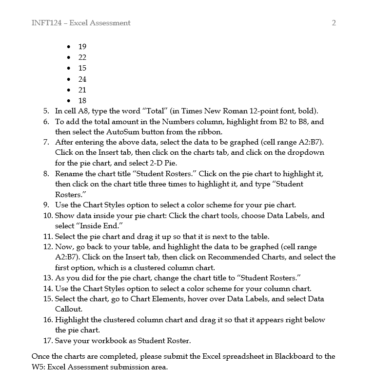
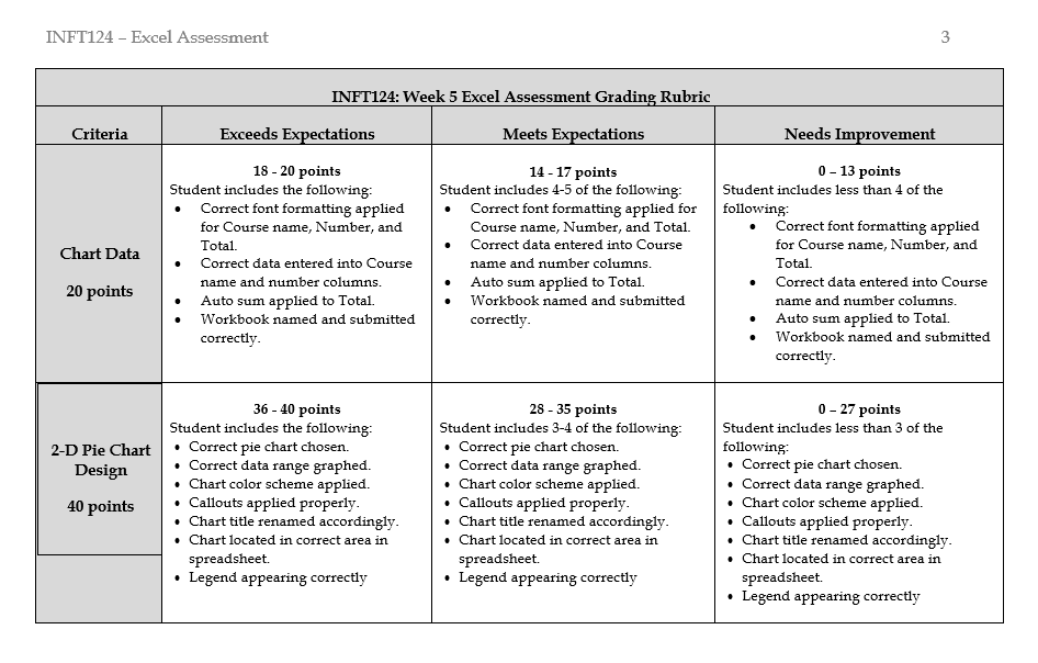
INFT124 -Excel Assessment 19 22 15 24 21 18 5. In cell A8, type the word "Total" (in Times New Roman 12-point font, bold). 6. To add the total amount in the Numbers column, highlight from B2 to B8, and then select the AutoSum button from the ribbon. 7. After entering the above data, select the data to be graphed (cell range A2:B7). Click on the Insert tab, then click on the charts tab, and click on the dropdown for the pie chart, and select 2-D Pie. 8. Rename the chart title "Student Rosters." Click on the pie chart to highlight it, then click on the chart title three times to highlight it, and type "Student Rosters." 9. Use the Chart Styles option to select a color scheme for your pie chart. 10. Show data inside your pie chart: Click the chart tools, choose Data Labels, and select "Inside End." 2 11. Select the pie chart and drag it up so that it is next to the table. 12. Now, go back to your table, and highlight the data to be graphed (cell range A2:B7). Click on the Insert tab, then click on Recommended Charts, and select the first option, which is a clustered column chart. 13. As you did for the pie chart, change the chart title to "Student Rosters." 14. Use the Chart Styles option to select a color scheme for your column chart. 15. Select the chart, go to Chart Elements, hover over Data Labels, and select Data Callout. 16. Highlight the clustered column chart and drag it so that it appears right below the pie chart. 17. Save your workbook as Student Roster. Once the charts are completed, please submit the Excel spreadsheet in Blackboard to the W5: Excel Assessment submission area. INFT124 - Excel Assessment Criteria Chart Data 20 points 2-D Pie Chart Design 40 points INFT124: Week 5 Excel Assessment Grading Rubric Exceeds Expectations 18-20 points Student includes the following: Correct font formatting applied for Course name, Number, and Total. Correct data entered into Course name and number columns. Auto sum applied to Total. Workbook named and submitted correctly. 36-40 points Student includes the following: Correct pie chart chosen. Correct data range graphed. Chart color scheme applied. Callouts applied properly. Chart title renamed accordingly. Chart located in correct area in spreadsheet. Legend appearing correctly Meets Expectations 14-17 points Student includes 4-5 of the following: Correct font formatting applied for Course name, Number, and Total. Correct data entered into Course name and number columns. Auto sum applied to Total. Workbook named and submitted correctly. 28-35 points Student includes 3-4 of the following: Correct pie chart chosen. Correct data range graphed. Chart color scheme applied. Callouts applied properly. Chart title renamed accordingly. Chart located in correct area in spreadsheet. Legend appearing correctly . 3 Needs Improvement 0-13 points Student includes less than 4 of the following: Correct font formatting applied for Course name, Number, and Total. Correct data entered into Course name and number columns. Auto sum applied to Total. Workbook named and submitted correctly. 0-27 points Student includes less than 3 of the following: Correct pie chart chosen. Correct data range graphed. Chart color scheme applied. Callouts applied properly. Chart title renamed accordingly. Chart located in correct area in spreadsheet. Legend appearing correctly INFT124 - Computing Skills Week 5 Excel Assessment This Assessment is part of the Workplace Assessments category, worth 20% of your grade. Deadline Due by the end of Week 5 at 11:59 pm, ET. Completing this Assessment will help you to meet the following: Course Outcome Create workplace-related documents, spreadsheets, and presentations using Office technology software Institutional Outcome Information Literacy and Communication - Utilize appropriate current technology and resources to locate and evaluate information needed to accomplish a goal, and then communicate findings in visual, written and/or oral formats. Directions In this assessment, you will create two graphs in an Excel spreadsheet: a pie chart and a column chart. You will follow the detailed steps below to organize the provided data and create the graphs. In your career, it's highly likely that you'll need to compile and showcase data for your boss, or while working on a team, or while preparing for a presentation. Learning these skills in Excel will make such tasks much easier. Once completed, please submit the Excel spreadsheet in Blackboard. Create a new Excel spreadsheet and enter the following information: 1. In cell A1 type "Course name" (Font should be Times New Roman 12-point font, bold). If these words are too big for the cell, click twice in between column headings A and B to resize the column. 2. In cell B1 type "Number" (Font should be Times New Roman 12-point font, bold). 3. Starting in cell A2 and working down this column, enter these course names (these can be any type font and size but be consistent, using the same font and size for all): COMM 104 HUSS 125 SOSC 226 PHIL 314 INFT 124 ACCT 210 4. Starting in cell B2 and working down this column, enter these quantities (these can be any type font and size, but again, be consistent): . INFT124 -Excel Assessment 19 22 15 24 21 18 5. In cell A8, type the word "Total" (in Times New Roman 12-point font, bold). 6. To add the total amount in the Numbers column, highlight from B2 to B8, and then select the AutoSum button from the ribbon. 7. After entering the above data, select the data to be graphed (cell range A2:B7). Click on the Insert tab, then click on the charts tab, and click on the dropdown for the pie chart, and select 2-D Pie. 8. Rename the chart title "Student Rosters." Click on the pie chart to highlight it, then click on the chart title three times to highlight it, and type "Student Rosters." 9. Use the Chart Styles option to select a color scheme for your pie chart. 10. Show data inside your pie chart: Click the chart tools, choose Data Labels, and select "Inside End." 2 11. Select the pie chart and drag it up so that it is next to the table. 12. Now, go back to your table, and highlight the data to be graphed (cell range A2:B7). Click on the Insert tab, then click on Recommended Charts, and select the first option, which is a clustered column chart. 13. As you did for the pie chart, change the chart title to "Student Rosters." 14. Use the Chart Styles option to select a color scheme for your column chart. 15. Select the chart, go to Chart Elements, hover over Data Labels, and select Data Callout. 16. Highlight the clustered column chart and drag it so that it appears right below the pie chart. 17. Save your workbook as Student Roster. Once the charts are completed, please submit the Excel spreadsheet in Blackboard to the W5: Excel Assessment submission area. INFT124 - Excel Assessment Criteria Chart Data 20 points 2-D Pie Chart Design 40 points INFT124: Week 5 Excel Assessment Grading Rubric Exceeds Expectations 18-20 points Student includes the following: Correct font formatting applied for Course name, Number, and Total. Correct data entered into Course name and number columns. Auto sum applied to Total. Workbook named and submitted correctly. 36-40 points Student includes the following: Correct pie chart chosen. Correct data range graphed. Chart color scheme applied. Callouts applied properly. Chart title renamed accordingly. Chart located in correct area in spreadsheet. Legend appearing correctly Meets Expectations 14-17 points Student includes 4-5 of the following: Correct font formatting applied for Course name, Number, and Total. Correct data entered into Course name and number columns. Auto sum applied to Total. Workbook named and submitted correctly. 28-35 points Student includes 3-4 of the following: Correct pie chart chosen. Correct data range graphed. Chart color scheme applied. Callouts applied properly. Chart title renamed accordingly. Chart located in correct area in spreadsheet. Legend appearing correctly . 3 Needs Improvement 0-13 points Student includes less than 4 of the following: Correct font formatting applied for Course name, Number, and Total. Correct data entered into Course name and number columns. Auto sum applied to Total. Workbook named and submitted correctly. 0-27 points Student includes less than 3 of the following: Correct pie chart chosen. Correct data range graphed. Chart color scheme applied. Callouts applied properly. Chart title renamed accordingly. Chart located in correct area in spreadsheet. Legend appearing correctly INFT124 - Computing Skills Week 5 Excel Assessment This Assessment is part of the Workplace Assessments category, worth 20% of your grade. Deadline Due by the end of Week 5 at 11:59 pm, ET. Completing this Assessment will help you to meet the following: Course Outcome Create workplace-related documents, spreadsheets, and presentations using Office technology software Institutional Outcome Information Literacy and Communication - Utilize appropriate current technology and resources to locate and evaluate information needed to accomplish a goal, and then communicate findings in visual, written and/or oral formats. Directions In this assessment, you will create two graphs in an Excel spreadsheet: a pie chart and a column chart. You will follow the detailed steps below to organize the provided data and create the graphs. In your career, it's highly likely that you'll need to compile and showcase data for your boss, or while working on a team, or while preparing for a presentation. Learning these skills in Excel will make such tasks much easier. Once completed, please submit the Excel spreadsheet in Blackboard. Create a new Excel spreadsheet and enter the following information: 1. In cell A1 type "Course name" (Font should be Times New Roman 12-point font, bold). If these words are too big for the cell, click twice in between column headings A and B to resize the column. 2. In cell B1 type "Number" (Font should be Times New Roman 12-point font, bold). 3. Starting in cell A2 and working down this column, enter these course names (these can be any type font and size but be consistent, using the same font and size for all): COMM 104 HUSS 125 SOSC 226 PHIL 314 INFT 124 ACCT 210 4. Starting in cell B2 and working down this column, enter these quantities (these can be any type font and size, but again, be consistent): .

Answer rating: 100% (QA)

Lets break down the instructions step by step Entering Course Names and Numbers In cell A1 type Cour... View the full answer