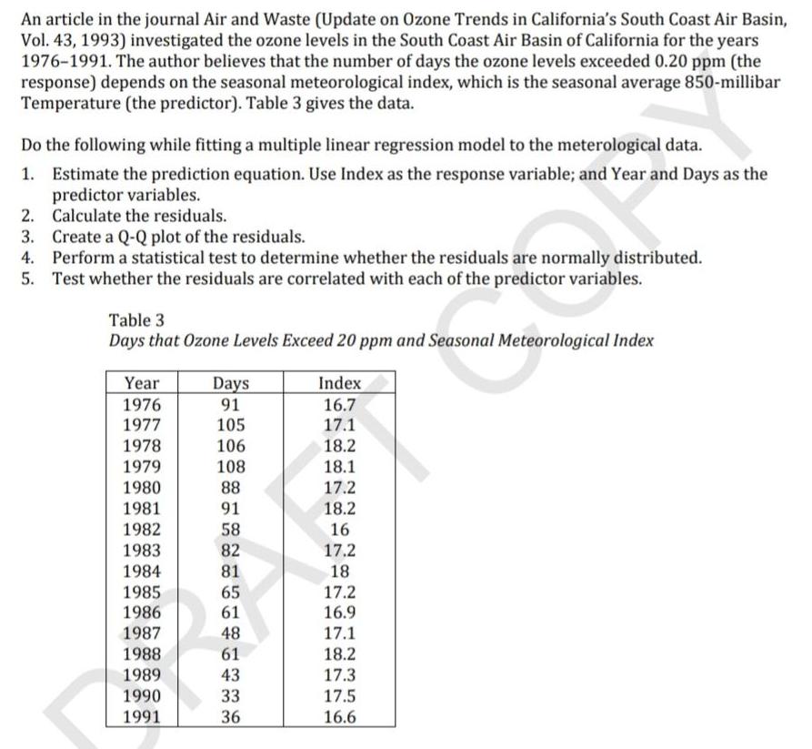
An article in the journal Air and Waste (Update on Ozone Trends in California's South Coast...

 

Transcribed Image Text:

An article in the journal Air and Waste (Update on Ozone Trends in California's South Coast Air Basin, Vol. 43, 1993) investigated the ozone levels in the South Coast Air Basin of California for the years 1976-1991. The author believes that the number of days the ozone levels exceeded 0.20 ppm (the response) depends on the seasonal meteorological index, which is the seasonal average 850-millibar Temperature (the predictor). Table 3 gives the data. Do the following while fitting a multiple linear regression model to the meterological data. 1. Estimate the prediction equation. Use Index as the response variable; and Year and Days as the predictor variables. Calculate the residuals. 2. 3. Create a Q-Q plot of the residuals. 4. Perform a statistical test to determine whether the residuals are normally distributed. 5. Test whether the residuals are correlated with each of the predictor variables. Table 3 Days that Ozone Levels Exceed 20 ppm and Seasonal Meteorological Index Year 1976 1977 1978 1979 1980 1981 1982 1983 1984 1985 1986 1987 1988 1989 1990 1991 Days 91 105 106 108 88 91 58 82 81 65 61 48 61 43 33 36 Index 16.7 17.1 18.2 18.1 17.2 18.2 16 17.2 18 17.2 16.9 17.1 18.2 17.3 17.5 16.6 An article in the journal Air and Waste (Update on Ozone Trends in California's South Coast Air Basin, Vol. 43, 1993) investigated the ozone levels in the South Coast Air Basin of California for the years 1976-1991. The author believes that the number of days the ozone levels exceeded 0.20 ppm (the response) depends on the seasonal meteorological index, which is the seasonal average 850-millibar Temperature (the predictor). Table 3 gives the data. Do the following while fitting a multiple linear regression model to the meterological data. 1. Estimate the prediction equation. Use Index as the response variable; and Year and Days as the predictor variables. Calculate the residuals. 2. 3. Create a Q-Q plot of the residuals. 4. Perform a statistical test to determine whether the residuals are normally distributed. 5. Test whether the residuals are correlated with each of the predictor variables. Table 3 Days that Ozone Levels Exceed 20 ppm and Seasonal Meteorological Index Year 1976 1977 1978 1979 1980 1981 1982 1983 1984 1985 1986 1987 1988 1989 1990 1991 Days 91 105 106 108 88 91 58 82 81 65 61 48 61 43 33 36 Index 16.7 17.1 18.2 18.1 17.2 18.2 16 17.2 18 17.2 16.9 17.1 18.2 17.3 17.5 16.6

Answer rating: 100% (QA)

1 Estimate the prediction equation Use Index as the response variable and Year and Days as the predictor variables The multiple linear regression equa... View the full answer