

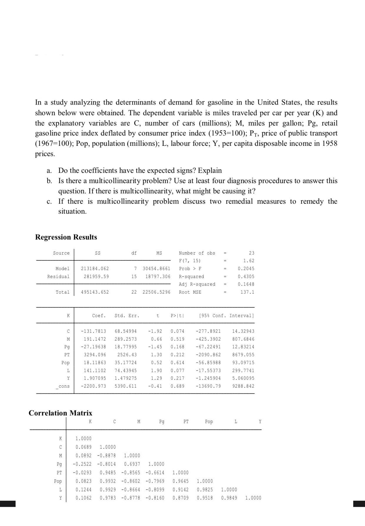
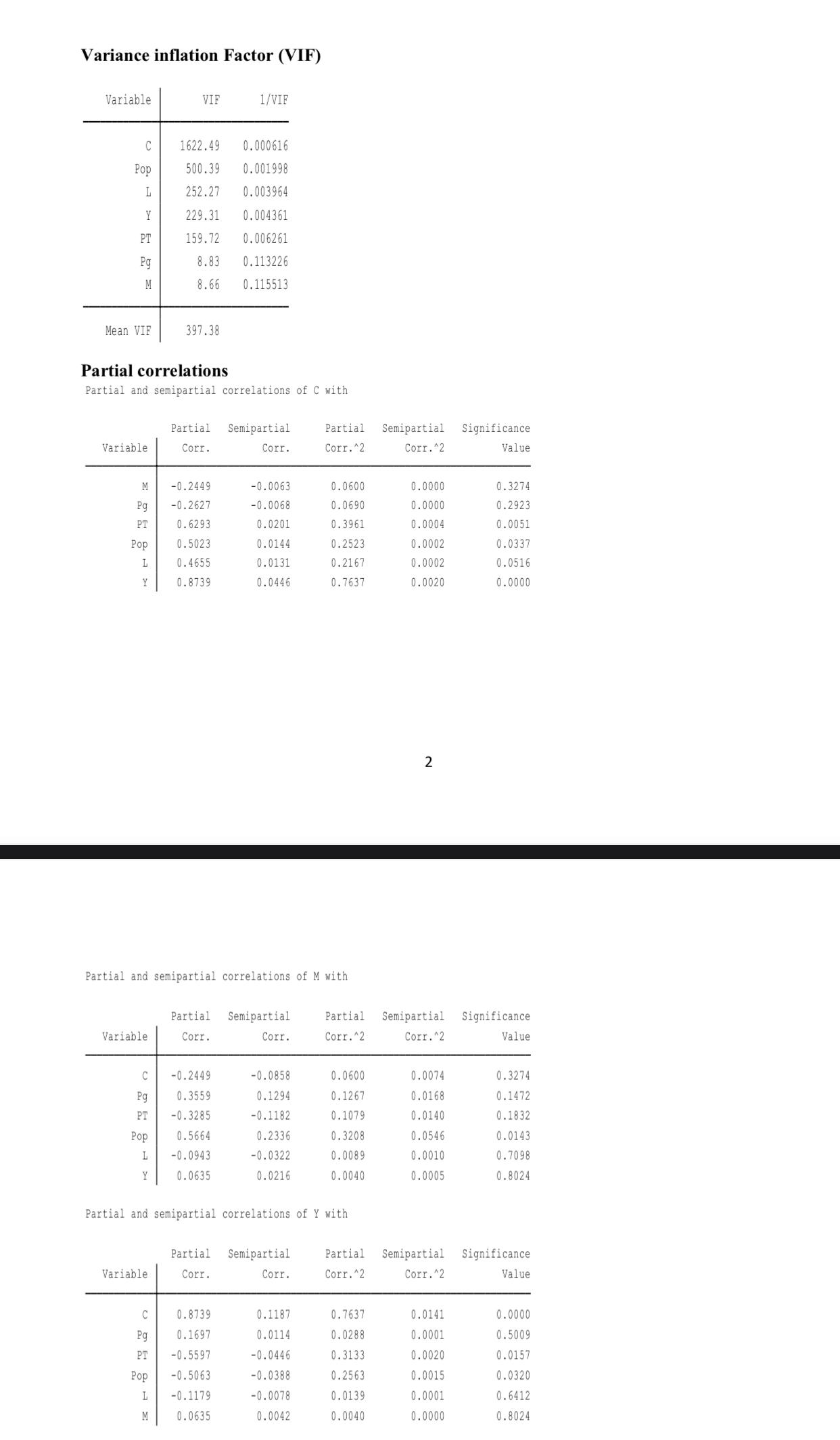
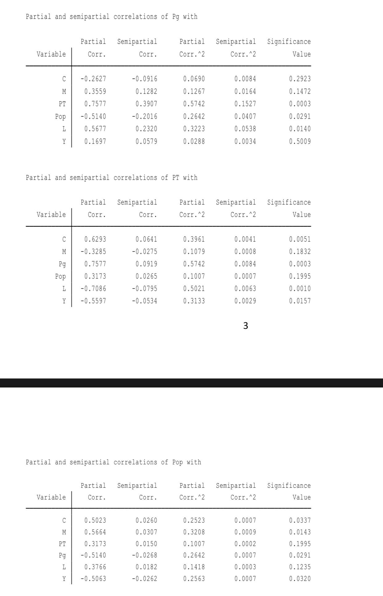
In a study analyzing the determinants of demand for gasoline in the United States, the results...
Fantastic news! We've Found the answer you've been seeking!
Question:
Transcribed Image Text:
In a study analyzing the determinants of demand for gasoline in the United States, the results shown below were obtained. The dependent variable is miles traveled per car per year (K) and the explanatory variables are C, number of cars (millions); M, miles per gallon; Pg, retail gasoline price index deflated by consumer price index (1953=100); PT, price of public transport (1967=100); Pop, population (millions); L, labour force; Y, per capita disposable income in 1958 prices. a. Do the coefficients have the expected signs? Explain b. Is there a multicollinearity problem? Use at least four diagnosis procedures to answer this question. If there is multicollinearity, what might be causing it? c. If there is multicollinearity problem discuss two remedial measures to remedy the situation. Regression Results Source Model Residual Total K Pop L Y cons K C M Pg PT C M Pg PT Pop L Y 213184.062 281959.59 SS 495143.652 Correlation Matrix Coef. K df -131.7813 68.54994 191.1472 289.2573 -27.19638 18.77995 3294.096 2526.43 18.11863 35.17724 141.1102 74.43945 47927 5390.611 9070 -2200.973 C 7 30454.8661 15 18797.306 Std. Err. 22 22506.5296 MS M t -0.41 Number of obs F(7, 15) Prob> F R-squared Adj R-squared = Root MSE -1.92 0.074 0.66 0.519 -1.45 0.168 1.30 0.212 0.52 0.614 1.90 0.077 217 0.689 Pg P> |t| PT -277.8921 -425.3902 -67.22491 -2090.862 -56.85988 -17.55373 -13690.79 = Pop = = = [95% Conf. Interval] 23 1.62 0.2045 0.4305 0.1648 137.1 14.32943 807.6846 12.83214 8679.055 93.09715 299.7741 L 9288.842 1.0000 0.0689 1.0000 0.0892 -0.8878 1.0000 -0.2522 -0.8014 0.6937 1.0000 -0.0293 0.9485 -0.8565 -0.6614 1.0000 0.0823 0.9932 -0.8602 -0.7969 0.9645 1.0000 0.1244 0.9929 -0.8664 -0.8099 0.9142 0.9825 1.0000 0.1062 0.9783 -0.8778 -0.8160 0.8709 Y 0.9518 0.9849 1.0000 Variance inflation Factor (VIF) Variable C Pop L Y PT Pg M Mean VIF Variable. M Pg PT Pop L Y Partial correlations Partial and semipartial correlations of C with Variable. C Pg PT VIF Pop 1622.49 0.000616 500.39 0.001998 252.27 0.003964 229.31 0.004361 159.72 0.006261 8.83 0.113226 8.66 0.115513 397.38 Variable: -0.2449 0.3559 -0.3285 0.5664 L -0.0943 Y 0.0635 C Pg PT 1/VIF Partial Semipartial Corr. Corr. -0.2449 -0.2627 0.6293 0.5023 0.4655 0.8739 Partial and semipartial correlations of M with -0.0063 -0.0068 0.0201 0.0144 0.0131 0.0446 Partial Semipartial Corr. Corr. 0.8739 0.1697 -0.5597 Pop -0.5063 L -0.1179 M 0.0635 -0.0858 0.1294 -0.1182 0.2336 -0.0322 0.0216 Partial Semipartial Corr. Corr. Partial Semipartial Corr.^2 Corr.^2 0.0600 0.0690 0.3961 0.1187 0.0114 -0.0446 -0.0388 -0.0078 0.0042 0.2523 0.2167 0.7637 Partial and semipartial correlations of Y with 0.0600 0.1267 0.1079 0.3208 0.0089 0.0040 0.0000 0.0000 0.0004 0.0002 0.0002 0.0020 Partial Semipartial Significance Corr.^2 Corr.^2 0.7637 0.0288 0.3133 2 0.2563 0.0139 0.0040 0.0074 0.0168 0.0140 0.0546 0.0010 0.0005 Significance Value 0.0141 0.0001 0.0020 0.0015 0.0001 0.0000 0.3274 0.2923 0.0051 0.0337 0.0516 0.0000 Partial Semipartial Significance. Corr.^2 Corr.^2 Value 0.3274 0.1472 0.1832 0.0143 0.7098 0.8024 Value 0.0000 0.5009 0.0157 0.0320 0.6412 0.8024 Partial and semipartial correlations of Pg with Variable C M PT Pop L Y Variable C M Pg Pop Partial Semipartial Corr. Corr. -0.2627 0.3559 0.7577 -0.5140 0.5677 0.1697 Partial and semipartial correlations of PT with Variable 0.6293 -0.3285 0.7577 0.3173 L -0.7086 Y -0.5597 C M Partial Corr. -0.0916 0.1282 0.3907 -0.2016 0.2320 0.0579 0.5023 0.5664 PT 0.3173 Pg -0.5140 L 0.3766 Y -0.5063 Semipartial Corr. 0.0641 -0.0275 0.0919 0.0265 -0.0795 -0.0534 Partial Semipartial Corr. Corr. Partial Semipartial Significance Corr.^2 Corr.^2 0.0690 0.1267 0.5742 0.2642 0.3223 0.0288 Partial and semipartial correlations of Pop with 0.0260 0.0307 0.0150 -0.0268 0.0182 -0.0262 0.3961 0.1079 0.5742 0.1007 0.5021 0.3133 Partial Semipartial Significance Corr.^2 Corr.^2 0.0084 0.0164 0.1527 0.0407 0.0538 0.0034 0.2523 0.3208 0.1007 0.2642 0.1418 0.2563 0.0041 0.0008 0.0084 0.0007 0.0063 0.0029 3 Partial Semipartial Corr.^2 Corr.^2 Value 0.0007 0.0009 0.0002 0.0007 0.0003 0.0007 0.2923 0.1472 0.0003 0.0291 0.0140 0.5009 Value 0.0051 0.1832 0.0003 0.1995 0.0010 0.0157 Significance Value 0.0337 0.0143 0.1995 0.0291 0.1235 0.0320 In a study analyzing the determinants of demand for gasoline in the United States, the results shown below were obtained. The dependent variable is miles traveled per car per year (K) and the explanatory variables are C, number of cars (millions); M, miles per gallon; Pg, retail gasoline price index deflated by consumer price index (1953=100); PT, price of public transport (1967=100); Pop, population (millions); L, labour force; Y, per capita disposable income in 1958 prices. a. Do the coefficients have the expected signs? Explain b. Is there a multicollinearity problem? Use at least four diagnosis procedures to answer this question. If there is multicollinearity, what might be causing it? c. If there is multicollinearity problem discuss two remedial measures to remedy the situation. Regression Results Source Model Residual Total K Pop L Y cons K C M Pg PT C M Pg PT Pop L Y 213184.062 281959.59 SS 495143.652 Correlation Matrix Coef. K df -131.7813 68.54994 191.1472 289.2573 -27.19638 18.77995 3294.096 2526.43 18.11863 35.17724 141.1102 74.43945 47927 5390.611 9070 -2200.973 C 7 30454.8661 15 18797.306 Std. Err. 22 22506.5296 MS M t -0.41 Number of obs F(7, 15) Prob> F R-squared Adj R-squared = Root MSE -1.92 0.074 0.66 0.519 -1.45 0.168 1.30 0.212 0.52 0.614 1.90 0.077 217 0.689 Pg P> |t| PT -277.8921 -425.3902 -67.22491 -2090.862 -56.85988 -17.55373 -13690.79 = Pop = = = [95% Conf. Interval] 23 1.62 0.2045 0.4305 0.1648 137.1 14.32943 807.6846 12.83214 8679.055 93.09715 299.7741 L 9288.842 1.0000 0.0689 1.0000 0.0892 -0.8878 1.0000 -0.2522 -0.8014 0.6937 1.0000 -0.0293 0.9485 -0.8565 -0.6614 1.0000 0.0823 0.9932 -0.8602 -0.7969 0.9645 1.0000 0.1244 0.9929 -0.8664 -0.8099 0.9142 0.9825 1.0000 0.1062 0.9783 -0.8778 -0.8160 0.8709 Y 0.9518 0.9849 1.0000 Variance inflation Factor (VIF) Variable C Pop L Y PT Pg M Mean VIF Variable. M Pg PT Pop L Y Partial correlations Partial and semipartial correlations of C with Variable. C Pg PT VIF Pop 1622.49 0.000616 500.39 0.001998 252.27 0.003964 229.31 0.004361 159.72 0.006261 8.83 0.113226 8.66 0.115513 397.38 Variable: -0.2449 0.3559 -0.3285 0.5664 L -0.0943 Y 0.0635 C Pg PT 1/VIF Partial Semipartial Corr. Corr. -0.2449 -0.2627 0.6293 0.5023 0.4655 0.8739 Partial and semipartial correlations of M with -0.0063 -0.0068 0.0201 0.0144 0.0131 0.0446 Partial Semipartial Corr. Corr. 0.8739 0.1697 -0.5597 Pop -0.5063 L -0.1179 M 0.0635 -0.0858 0.1294 -0.1182 0.2336 -0.0322 0.0216 Partial Semipartial Corr. Corr. Partial Semipartial Corr.^2 Corr.^2 0.0600 0.0690 0.3961 0.1187 0.0114 -0.0446 -0.0388 -0.0078 0.0042 0.2523 0.2167 0.7637 Partial and semipartial correlations of Y with 0.0600 0.1267 0.1079 0.3208 0.0089 0.0040 0.0000 0.0000 0.0004 0.0002 0.0002 0.0020 Partial Semipartial Significance Corr.^2 Corr.^2 0.7637 0.0288 0.3133 2 0.2563 0.0139 0.0040 0.0074 0.0168 0.0140 0.0546 0.0010 0.0005 Significance Value 0.0141 0.0001 0.0020 0.0015 0.0001 0.0000 0.3274 0.2923 0.0051 0.0337 0.0516 0.0000 Partial Semipartial Significance. Corr.^2 Corr.^2 Value 0.3274 0.1472 0.1832 0.0143 0.7098 0.8024 Value 0.0000 0.5009 0.0157 0.0320 0.6412 0.8024 Partial and semipartial correlations of Pg with Variable C M PT Pop L Y Variable C M Pg Pop Partial Semipartial Corr. Corr. -0.2627 0.3559 0.7577 -0.5140 0.5677 0.1697 Partial and semipartial correlations of PT with Variable 0.6293 -0.3285 0.7577 0.3173 L -0.7086 Y -0.5597 C M Partial Corr. -0.0916 0.1282 0.3907 -0.2016 0.2320 0.0579 0.5023 0.5664 PT 0.3173 Pg -0.5140 L 0.3766 Y -0.5063 Semipartial Corr. 0.0641 -0.0275 0.0919 0.0265 -0.0795 -0.0534 Partial Semipartial Corr. Corr. Partial Semipartial Significance Corr.^2 Corr.^2 0.0690 0.1267 0.5742 0.2642 0.3223 0.0288 Partial and semipartial correlations of Pop with 0.0260 0.0307 0.0150 -0.0268 0.0182 -0.0262 0.3961 0.1079 0.5742 0.1007 0.5021 0.3133 Partial Semipartial Significance Corr.^2 Corr.^2 0.0084 0.0164 0.1527 0.0407 0.0538 0.0034 0.2523 0.3208 0.1007 0.2642 0.1418 0.2563 0.0041 0.0008 0.0084 0.0007 0.0063 0.0029 3 Partial Semipartial Corr.^2 Corr.^2 Value 0.0007 0.0009 0.0002 0.0007 0.0003 0.0007 0.2923 0.1472 0.0003 0.0291 0.0140 0.5009 Value 0.0051 0.1832 0.0003 0.1995 0.0010 0.0157 Significance Value 0.0337 0.0143 0.1995 0.0291 0.1235 0.0320
Expert Answer:
Answer rating: 100% (QA)
a Coefficient Estimated Coefficient Estimated Variable Std Error tStatistic Probt C 5618184 0645573 ... View the full answer

Related Book For 

College Mathematics for Business Economics Life Sciences and Social Sciences
ISBN: 978-0321614001
12th edition
Authors: Raymond A. Barnett, Michael R. Ziegler, Karl E. Byleen
Posted Date:
Students also viewed these economics questions
-
1. If a and b denote the vectors OA and OB, indicate on the same diagram the vectors OC and OD denoted by a+ b and a- b. Draw on another diagram the vector OE denoted by a +2b. 2. ABCD is a square...
-
The project is about cyber Ethics, please read the pdf document to have an idea about it. Needs to have materials from Cyber Ethics. you can also use these links for some references.
-
Please read the description of the project before responding!!! hello, i am looking for an algebra expert for two tasks. the first task is for a review for an algebra final. i need to get a 100% on...
-
On June 15, 2020, Smithson Foods purchased $1,000,000 of 2.5 percent corporate bonds at par and designated them as availableforsale investments. On December 31, 2020, Smithsons yearend, the bonds are...
-
Eight subjects were weighed before and after a new three-week healthy diet. At the 0.05 level of significance, can it be concluded that a difference in weight resulted? (Weights are in pounds.)...
-
Why are weighted-average ordinary shares used in EPS calculations?
-
How many degrees of freedom are there? Exercises 49 refer to the following data: Electric motors are assembled on four different production lines. Random samples of motors are taken from each line...
-
A graphical approach was used to solve the following LP model in Problem 2-15: Maximize profit = $4X + $3T Subject to the constraints 3XY 27 X, Y >0
-
Required: What were the amounts in the beginning Finished Goods and beginning Work - in - Process accounts for Year 3 ? O Leary incurred direct materials costs of $ 5 7 , 0 0 0 and used an additional...
-
During 2008 the US economy stopped growing and began to shrink. Table 1.25 gives quarterly data on the US Gross Domestic Product (GDP), which measures the size of the economy. (a) Estimate the...
-
Continue with the version of the two-period consumption model discussed in question (4). (a) Calculate the present value of the consumer's tax expenditures. (b) Suppose that the government redcest...
-
What prevents the person who opens incoming mail from being able to abstract cash collections from customers?
-
Select the best answer for each of the following situations and give reasons for your choice. a. You have been assigned to the year-end audit of a financial institution and are planning the timing of...
-
Evaluate the following quotation: "Every business, large or small, should have an annual audit by a CPA firm. To forgo an audit because of its cost is false economy."
-
The first SAS issued was substantially larger and different in coverage from all the following ones. What explains this difference?
-
Your CPA firm has been requested to perform a peer review of the firm of William & Stafford. What is involved in the performance of such an engagement? Discuss.
-
1. Determine the amount earned on $11 800 at 8.4% per year, compounded quarterly, for 14 years. P = i = n = 2. It is Jerry's 14th birthday and his parents plan to invest some money so that they will...
-
Flicker, Inc., a closely held corporation, acquired a passive activity this year. Gross income from operations of the activity was $160,000. Operating expenses, not including depreciation, were...
-
Most appliance manufacturers produce conventional and energy-efficient models. The energy-efficient models are more expensive to make but cheaper to operate. The costs of purchasing and operating a...
-
Solve problem 5.x + 2 > 1
-
Repeat Problem 44 if the profit on a five-speed bicycle increases from $70 to $110 and all other data remain the same. If the slack associated with any problem constraint is nonzero, find it.
-
A pair of \(20^{\circ}\) full involute spur gears having 40 and 60 teeth of module \(4 \mathrm{~mm}\) are in mesh. The smaller gear rotates at \(1440 \mathrm{rpm}\). Find (a) sliding velocity at...
-
Calculate the minimum number of teeth on a pinion to avoid interference to have a speed ratio of 2.5:1. The pressure angle is \(20^{\circ}\) and addendum of one module of gear may be used.
-
The path of contact in involute gears is (a) a straight line (b) involute path (c) curved path (d) circle.

Study smarter with the SolutionInn App