

The Oceanside Garden Nursery buys flowering plants in four-inch pots for $1.50 each and sells them...
Fantastic news! We've Found the answer you've been seeking!
Question:


Transcribed Image Text:
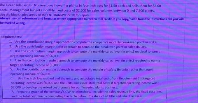
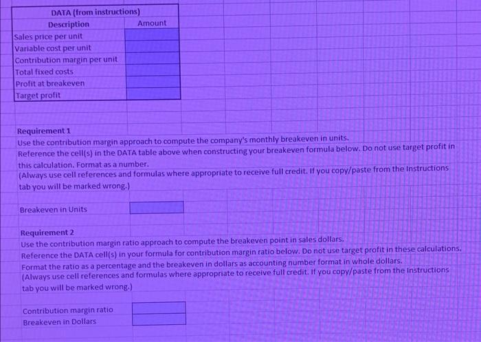
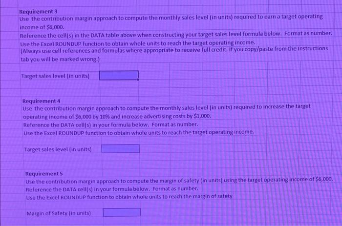
The Oceanside Garden Nursery buys flowering plants in four-inch pots for $1.50 each and sells them for $3.00 each. Management budgets monthly fixed costs of $2,600 for sales volumes between 0 and 7,500 plants. Use the blue shaded areas on the ENTERANSWERS tab for inputs. Always use cell references and formulas where appropriate to receive full credit. If you copy/paste from the Instructions tab you will be marked wrong. Requirements: 1. Use the contribution margin approach to compute the company's monthly breakeven point in units. 2. Use the contribution margin ratio approach to compute the breakeven point in sales dollars. 3. Use the contribution margin approach to compute the monthly sales level (in units) required to earn a target operating income of $6,000. 4. Use the contribution margin approach to compute the monthly sales level (in units) required to earn a target operating income of S6,000. 5. Use the contribution margin approach to compute the margin of safety (in units) using the target operating income of $6,000. Use the high low method and the units and associated total costs from Requirement 3 If targeted operating income was $6,000 and the units and associated total costs If targeted operating income was $7,000 to develop the mixed cost formula for our flowering olants business. 7. Prepare a graph of the company's CVP relationships. Include the sales revenue line, the fixed cost line, and the total cost line by completing the table below. Create a chart title and label the axes. 6. DATA (from instructions) Description Amount Sales price per unit Variable cost per unit Contribution margin per unit Total fixed costs Profit at breakeven Target profit Requirement 1 Use the contribution margin approach to compute the company's monthly breakeven in units. Reference the cell(s) in the DATA table above when constructing your breakeven formula below. Do not use target profit in this calculation. Format as a number. (Always use cell references and formulas where appropriate to receive full credit. If you copy/paste from the Instructions tab you will be marked wrong.-) Breakeven in Units Requirement 2 Use the contribution margin ratio approach to compute the breakeven point in sales dollars. Reference the DATA cell(s) in your formula for contribution margin ratio below. Do not use target profit in these calculations. Format the ratio as a percentage and the breakeven in dollars as accounting number format in whole dollars. (Always use cell references and formulas where appropriate to receive full credit. If you copy/paste from the Instructions tab you will be marked wrong.) Contribution margin ratio Breakeven in Dollars Requirement 3 Use the contribution margin approach to compute the monthly sales level (in units) required to earn a target operating income of $6,000. Reference the cell(s) in the DATA table above when constructing your target sales level formula below. Format as number. Use the Excel ROUNDUP function to obtain whole units to reach the target operating income. (Always use cell references and formulas where appropriate to receive full credit. If you copy/paste from the Instructions tab you will be marked wrong.) Target sales level (in units) Requirement 4 Use the contribution margin approach to compute the monthly sales level (in units) required to increase the target operating income of $6,000 by 10% and increase advertising costs by $1,000. Reference the DATA cell(s) in your formula below. Format as number. Use the Excel ROUNDUP function to obtain whole units to reach the target operating income. Target sales level (in units) Requirement 5 Use the contribution margin approach to compute the margin of safety (in units) using the target operating income of $6,000. Reference the DATA cell(s) in your formula below. Format as number. Use the Excel ROUNDUP function to obtain whole units to reach the margin of safety Margin of Safety (in units) 53 Requirement 6 Use the high low method and the units and associated total costs from Requirement 3 if targeted operating income was $6,000 and the units and associated total costs if targeted operating income was $7,000 to develop the mixed cost formula for our flowering plants business. Reference the DATA cell(s) in your formula below. Format appropriately. 54 55 56 57 High Low Method Step 1-Variable cost per unit 58 59 60 61 Step 2- Fixed Cost 62 63 Step 3- Mixed Cost Formula 64 65 66 HINTS 67 Cell | Hint: C4:C9 | Enter the appropriate numeric values given on the Instructions tab. Use an equal sign (-) and the appropriate cells previously completed in the DATA table to calculate the values that are not directly given on the Instructions tab. Do not use equal sign 68 (-) 69 C35 | Use the function =ROUNDUP( ), to calculate the target sales level. 70 C43 | Use the function =ROUNDUP( ), to calculate the margin of safety. 71 72 To create the graph: 1. Once the data are entered, select the following four rows using the CTRL key to select non-contiguous cells: Volume, Revenue, Fixed Costs, and Total Cost. This means you select Rows 25, 26, 28 and 29; Column B through Column O. 2. Select the Insert tab, select "scatter or bubble chart" from the chart menu, then click "Scatter with Smooth Lines and Markers." Right click and move the chart to the Graph tab. Formu Dev Iert Draw Page Layout Vw Store Une Colun Recommendel Charts utration Tecommended table Potlable 30 Map PeChat My Add ie O Scatter Sp Cuse Dooumebos Scatter with Semooth Lines andMarken Uu this chathpe to Compare at at two of als or pas uf data 3. On the Design tab, select "Add Chart Element" then select "Chart Title" then select "Above Chart." Add the title "Breakeven." Toml fum Cve MrOwE G Dege Der 4. On the Design tab, select "Add Chart Element", then select "Axis Titles" and then select "Primary Horizontal"; label the x axis as "Units". Dre PageLa Farmule Dele Cee Deg foma Mome PPRT Cange Color Emmant Leyiut oune Chat Me Con The Oceanside Garden Nursery buys flowering plants in four-inch pots for $1.50 each and sells them for $3.00 each. Management budgets monthly fixed costs of $2,600 for sales volumes between 0 and 7,500 plants. Use the blue shaded areas on the ENTERANSWERS tab for inputs. Always use cell references and formulas where appropriate to receive full credit. If you copy/paste from the Instructions tab you will be marked wrong. Requirements: 1. Use the contribution margin approach to compute the company's monthly breakeven point in units. 2. Use the contribution margin ratio approach to compute the breakeven point in sales dollars. 3. Use the contribution margin approach to compute the monthly sales level (in units) required to earn a target operating income of $6,000. 4. Use the contribution margin approach to compute the monthly sales level (in units) required to earn a target operating income of S6,000. 5. Use the contribution margin approach to compute the margin of safety (in units) using the target operating income of $6,000. Use the high low method and the units and associated total costs from Requirement 3 If targeted operating income was $6,000 and the units and associated total costs If targeted operating income was $7,000 to develop the mixed cost formula for our flowering olants business. 7. Prepare a graph of the company's CVP relationships. Include the sales revenue line, the fixed cost line, and the total cost line by completing the table below. Create a chart title and label the axes. 6. DATA (from instructions) Description Amount Sales price per unit Variable cost per unit Contribution margin per unit Total fixed costs Profit at breakeven Target profit Requirement 1 Use the contribution margin approach to compute the company's monthly breakeven in units. Reference the cell(s) in the DATA table above when constructing your breakeven formula below. Do not use target profit in this calculation. Format as a number. (Always use cell references and formulas where appropriate to receive full credit. If you copy/paste from the Instructions tab you will be marked wrong.-) Breakeven in Units Requirement 2 Use the contribution margin ratio approach to compute the breakeven point in sales dollars. Reference the DATA cell(s) in your formula for contribution margin ratio below. Do not use target profit in these calculations. Format the ratio as a percentage and the breakeven in dollars as accounting number format in whole dollars. (Always use cell references and formulas where appropriate to receive full credit. If you copy/paste from the Instructions tab you will be marked wrong.) Contribution margin ratio Breakeven in Dollars Requirement 3 Use the contribution margin approach to compute the monthly sales level (in units) required to earn a target operating income of $6,000. Reference the cell(s) in the DATA table above when constructing your target sales level formula below. Format as number. Use the Excel ROUNDUP function to obtain whole units to reach the target operating income. (Always use cell references and formulas where appropriate to receive full credit. If you copy/paste from the Instructions tab you will be marked wrong.) Target sales level (in units) Requirement 4 Use the contribution margin approach to compute the monthly sales level (in units) required to increase the target operating income of $6,000 by 10% and increase advertising costs by $1,000. Reference the DATA cell(s) in your formula below. Format as number. Use the Excel ROUNDUP function to obtain whole units to reach the target operating income. Target sales level (in units) Requirement 5 Use the contribution margin approach to compute the margin of safety (in units) using the target operating income of $6,000. Reference the DATA cell(s) in your formula below. Format as number. Use the Excel ROUNDUP function to obtain whole units to reach the margin of safety Margin of Safety (in units) 53 Requirement 6 Use the high low method and the units and associated total costs from Requirement 3 if targeted operating income was $6,000 and the units and associated total costs if targeted operating income was $7,000 to develop the mixed cost formula for our flowering plants business. Reference the DATA cell(s) in your formula below. Format appropriately. 54 55 56 57 High Low Method Step 1-Variable cost per unit 58 59 60 61 Step 2- Fixed Cost 62 63 Step 3- Mixed Cost Formula 64 65 66 HINTS 67 Cell | Hint: C4:C9 | Enter the appropriate numeric values given on the Instructions tab. Use an equal sign (-) and the appropriate cells previously completed in the DATA table to calculate the values that are not directly given on the Instructions tab. Do not use equal sign 68 (-) 69 C35 | Use the function =ROUNDUP( ), to calculate the target sales level. 70 C43 | Use the function =ROUNDUP( ), to calculate the margin of safety. 71 72 To create the graph: 1. Once the data are entered, select the following four rows using the CTRL key to select non-contiguous cells: Volume, Revenue, Fixed Costs, and Total Cost. This means you select Rows 25, 26, 28 and 29; Column B through Column O. 2. Select the Insert tab, select "scatter or bubble chart" from the chart menu, then click "Scatter with Smooth Lines and Markers." Right click and move the chart to the Graph tab. Formu Dev Iert Draw Page Layout Vw Store Une Colun Recommendel Charts utration Tecommended table Potlable 30 Map PeChat My Add ie O Scatter Sp Cuse Dooumebos Scatter with Semooth Lines andMarken Uu this chathpe to Compare at at two of als or pas uf data 3. On the Design tab, select "Add Chart Element" then select "Chart Title" then select "Above Chart." Add the title "Breakeven." Toml fum Cve MrOwE G Dege Der 4. On the Design tab, select "Add Chart Element", then select "Axis Titles" and then select "Primary Horizontal"; label the x axis as "Units". Dre PageLa Farmule Dele Cee Deg foma Mome PPRT Cange Color Emmant Leyiut oune Chat Me Con The Oceanside Garden Nursery buys flowering plants in four-inch pots for $1.50 each and sells them for $3.00 each. Management budgets monthly fixed costs of $2,600 for sales volumes between 0 and 7,500 plants. Use the blue shaded areas on the ENTERANSWERS tab for inputs. Always use cell references and formulas where appropriate to receive full credit. If you copy/paste from the Instructions tab you will be marked wrong. Requirements: 1. Use the contribution margin approach to compute the company's monthly breakeven point in units. 2. Use the contribution margin ratio approach to compute the breakeven point in sales dollars. 3. Use the contribution margin approach to compute the monthly sales level (in units) required to earn a target operating income of $6,000. 4. Use the contribution margin approach to compute the monthly sales level (in units) required to earn a target operating income of S6,000. 5. Use the contribution margin approach to compute the margin of safety (in units) using the target operating income of $6,000. Use the high low method and the units and associated total costs from Requirement 3 If targeted operating income was $6,000 and the units and associated total costs If targeted operating income was $7,000 to develop the mixed cost formula for our flowering olants business. 7. Prepare a graph of the company's CVP relationships. Include the sales revenue line, the fixed cost line, and the total cost line by completing the table below. Create a chart title and label the axes. 6. DATA (from instructions) Description Amount Sales price per unit Variable cost per unit Contribution margin per unit Total fixed costs Profit at breakeven Target profit Requirement 1 Use the contribution margin approach to compute the company's monthly breakeven in units. Reference the cell(s) in the DATA table above when constructing your breakeven formula below. Do not use target profit in this calculation. Format as a number. (Always use cell references and formulas where appropriate to receive full credit. If you copy/paste from the Instructions tab you will be marked wrong.-) Breakeven in Units Requirement 2 Use the contribution margin ratio approach to compute the breakeven point in sales dollars. Reference the DATA cell(s) in your formula for contribution margin ratio below. Do not use target profit in these calculations. Format the ratio as a percentage and the breakeven in dollars as accounting number format in whole dollars. (Always use cell references and formulas where appropriate to receive full credit. If you copy/paste from the Instructions tab you will be marked wrong.) Contribution margin ratio Breakeven in Dollars Requirement 3 Use the contribution margin approach to compute the monthly sales level (in units) required to earn a target operating income of $6,000. Reference the cell(s) in the DATA table above when constructing your target sales level formula below. Format as number. Use the Excel ROUNDUP function to obtain whole units to reach the target operating income. (Always use cell references and formulas where appropriate to receive full credit. If you copy/paste from the Instructions tab you will be marked wrong.) Target sales level (in units) Requirement 4 Use the contribution margin approach to compute the monthly sales level (in units) required to increase the target operating income of $6,000 by 10% and increase advertising costs by $1,000. Reference the DATA cell(s) in your formula below. Format as number. Use the Excel ROUNDUP function to obtain whole units to reach the target operating income. Target sales level (in units) Requirement 5 Use the contribution margin approach to compute the margin of safety (in units) using the target operating income of $6,000. Reference the DATA cell(s) in your formula below. Format as number. Use the Excel ROUNDUP function to obtain whole units to reach the margin of safety Margin of Safety (in units) 53 Requirement 6 Use the high low method and the units and associated total costs from Requirement 3 if targeted operating income was $6,000 and the units and associated total costs if targeted operating income was $7,000 to develop the mixed cost formula for our flowering plants business. Reference the DATA cell(s) in your formula below. Format appropriately. 54 55 56 57 High Low Method Step 1-Variable cost per unit 58 59 60 61 Step 2- Fixed Cost 62 63 Step 3- Mixed Cost Formula 64 65 66 HINTS 67 Cell | Hint: C4:C9 | Enter the appropriate numeric values given on the Instructions tab. Use an equal sign (-) and the appropriate cells previously completed in the DATA table to calculate the values that are not directly given on the Instructions tab. Do not use equal sign 68 (-) 69 C35 | Use the function =ROUNDUP( ), to calculate the target sales level. 70 C43 | Use the function =ROUNDUP( ), to calculate the margin of safety. 71 72 To create the graph: 1. Once the data are entered, select the following four rows using the CTRL key to select non-contiguous cells: Volume, Revenue, Fixed Costs, and Total Cost. This means you select Rows 25, 26, 28 and 29; Column B through Column O. 2. Select the Insert tab, select "scatter or bubble chart" from the chart menu, then click "Scatter with Smooth Lines and Markers." Right click and move the chart to the Graph tab. Formu Dev Iert Draw Page Layout Vw Store Une Colun Recommendel Charts utration Tecommended table Potlable 30 Map PeChat My Add ie O Scatter Sp Cuse Dooumebos Scatter with Semooth Lines andMarken Uu this chathpe to Compare at at two of als or pas uf data 3. On the Design tab, select "Add Chart Element" then select "Chart Title" then select "Above Chart." Add the title "Breakeven." Toml fum Cve MrOwE G Dege Der 4. On the Design tab, select "Add Chart Element", then select "Axis Titles" and then select "Primary Horizontal"; label the x axis as "Units". Dre PageLa Farmule Dele Cee Deg foma Mome PPRT Cange Color Emmant Leyiut oune Chat Me Con The Oceanside Garden Nursery buys flowering plants in four-inch pots for $1.50 each and sells them for $3.00 each. Management budgets monthly fixed costs of $2,600 for sales volumes between 0 and 7,500 plants. Use the blue shaded areas on the ENTERANSWERS tab for inputs. Always use cell references and formulas where appropriate to receive full credit. If you copy/paste from the Instructions tab you will be marked wrong. Requirements: 1. Use the contribution margin approach to compute the company's monthly breakeven point in units. 2. Use the contribution margin ratio approach to compute the breakeven point in sales dollars. 3. Use the contribution margin approach to compute the monthly sales level (in units) required to earn a target operating income of $6,000. 4. Use the contribution margin approach to compute the monthly sales level (in units) required to earn a target operating income of S6,000. 5. Use the contribution margin approach to compute the margin of safety (in units) using the target operating income of $6,000. Use the high low method and the units and associated total costs from Requirement 3 If targeted operating income was $6,000 and the units and associated total costs If targeted operating income was $7,000 to develop the mixed cost formula for our flowering olants business. 7. Prepare a graph of the company's CVP relationships. Include the sales revenue line, the fixed cost line, and the total cost line by completing the table below. Create a chart title and label the axes. 6. DATA (from instructions) Description Amount Sales price per unit Variable cost per unit Contribution margin per unit Total fixed costs Profit at breakeven Target profit Requirement 1 Use the contribution margin approach to compute the company's monthly breakeven in units. Reference the cell(s) in the DATA table above when constructing your breakeven formula below. Do not use target profit in this calculation. Format as a number. (Always use cell references and formulas where appropriate to receive full credit. If you copy/paste from the Instructions tab you will be marked wrong.-) Breakeven in Units Requirement 2 Use the contribution margin ratio approach to compute the breakeven point in sales dollars. Reference the DATA cell(s) in your formula for contribution margin ratio below. Do not use target profit in these calculations. Format the ratio as a percentage and the breakeven in dollars as accounting number format in whole dollars. (Always use cell references and formulas where appropriate to receive full credit. If you copy/paste from the Instructions tab you will be marked wrong.) Contribution margin ratio Breakeven in Dollars Requirement 3 Use the contribution margin approach to compute the monthly sales level (in units) required to earn a target operating income of $6,000. Reference the cell(s) in the DATA table above when constructing your target sales level formula below. Format as number. Use the Excel ROUNDUP function to obtain whole units to reach the target operating income. (Always use cell references and formulas where appropriate to receive full credit. If you copy/paste from the Instructions tab you will be marked wrong.) Target sales level (in units) Requirement 4 Use the contribution margin approach to compute the monthly sales level (in units) required to increase the target operating income of $6,000 by 10% and increase advertising costs by $1,000. Reference the DATA cell(s) in your formula below. Format as number. Use the Excel ROUNDUP function to obtain whole units to reach the target operating income. Target sales level (in units) Requirement 5 Use the contribution margin approach to compute the margin of safety (in units) using the target operating income of $6,000. Reference the DATA cell(s) in your formula below. Format as number. Use the Excel ROUNDUP function to obtain whole units to reach the margin of safety Margin of Safety (in units) 53 Requirement 6 Use the high low method and the units and associated total costs from Requirement 3 if targeted operating income was $6,000 and the units and associated total costs if targeted operating income was $7,000 to develop the mixed cost formula for our flowering plants business. Reference the DATA cell(s) in your formula below. Format appropriately. 54 55 56 57 High Low Method Step 1-Variable cost per unit 58 59 60 61 Step 2- Fixed Cost 62 63 Step 3- Mixed Cost Formula 64 65 66 HINTS 67 Cell | Hint: C4:C9 | Enter the appropriate numeric values given on the Instructions tab. Use an equal sign (-) and the appropriate cells previously completed in the DATA table to calculate the values that are not directly given on the Instructions tab. Do not use equal sign 68 (-) 69 C35 | Use the function =ROUNDUP( ), to calculate the target sales level. 70 C43 | Use the function =ROUNDUP( ), to calculate the margin of safety. 71 72 To create the graph: 1. Once the data are entered, select the following four rows using the CTRL key to select non-contiguous cells: Volume, Revenue, Fixed Costs, and Total Cost. This means you select Rows 25, 26, 28 and 29; Column B through Column O. 2. Select the Insert tab, select "scatter or bubble chart" from the chart menu, then click "Scatter with Smooth Lines and Markers." Right click and move the chart to the Graph tab. Formu Dev Iert Draw Page Layout Vw Store Une Colun Recommendel Charts utration Tecommended table Potlable 30 Map PeChat My Add ie O Scatter Sp Cuse Dooumebos Scatter with Semooth Lines andMarken Uu this chathpe to Compare at at two of als or pas uf data 3. On the Design tab, select "Add Chart Element" then select "Chart Title" then select "Above Chart." Add the title "Breakeven." Toml fum Cve MrOwE G Dege Der 4. On the Design tab, select "Add Chart Element", then select "Axis Titles" and then select "Primary Horizontal"; label the x axis as "Units". Dre PageLa Farmule Dele Cee Deg foma Mome PPRT Cange Color Emmant Leyiut oune Chat Me Con The Oceanside Garden Nursery buys flowering plants in four-inch pots for $1.50 each and sells them for $3.00 each. Management budgets monthly fixed costs of $2,600 for sales volumes between 0 and 7,500 plants. Use the blue shaded areas on the ENTERANSWERS tab for inputs. Always use cell references and formulas where appropriate to receive full credit. If you copy/paste from the Instructions tab you will be marked wrong. Requirements: 1. Use the contribution margin approach to compute the company's monthly breakeven point in units. 2. Use the contribution margin ratio approach to compute the breakeven point in sales dollars. 3. Use the contribution margin approach to compute the monthly sales level (in units) required to earn a target operating income of $6,000. 4. Use the contribution margin approach to compute the monthly sales level (in units) required to earn a target operating income of S6,000. 5. Use the contribution margin approach to compute the margin of safety (in units) using the target operating income of $6,000. Use the high low method and the units and associated total costs from Requirement 3 If targeted operating income was $6,000 and the units and associated total costs If targeted operating income was $7,000 to develop the mixed cost formula for our flowering olants business. 7. Prepare a graph of the company's CVP relationships. Include the sales revenue line, the fixed cost line, and the total cost line by completing the table below. Create a chart title and label the axes. 6. DATA (from instructions) Description Amount Sales price per unit Variable cost per unit Contribution margin per unit Total fixed costs Profit at breakeven Target profit Requirement 1 Use the contribution margin approach to compute the company's monthly breakeven in units. Reference the cell(s) in the DATA table above when constructing your breakeven formula below. Do not use target profit in this calculation. Format as a number. (Always use cell references and formulas where appropriate to receive full credit. If you copy/paste from the Instructions tab you will be marked wrong.-) Breakeven in Units Requirement 2 Use the contribution margin ratio approach to compute the breakeven point in sales dollars. Reference the DATA cell(s) in your formula for contribution margin ratio below. Do not use target profit in these calculations. Format the ratio as a percentage and the breakeven in dollars as accounting number format in whole dollars. (Always use cell references and formulas where appropriate to receive full credit. If you copy/paste from the Instructions tab you will be marked wrong.) Contribution margin ratio Breakeven in Dollars Requirement 3 Use the contribution margin approach to compute the monthly sales level (in units) required to earn a target operating income of $6,000. Reference the cell(s) in the DATA table above when constructing your target sales level formula below. Format as number. Use the Excel ROUNDUP function to obtain whole units to reach the target operating income. (Always use cell references and formulas where appropriate to receive full credit. If you copy/paste from the Instructions tab you will be marked wrong.) Target sales level (in units) Requirement 4 Use the contribution margin approach to compute the monthly sales level (in units) required to increase the target operating income of $6,000 by 10% and increase advertising costs by $1,000. Reference the DATA cell(s) in your formula below. Format as number. Use the Excel ROUNDUP function to obtain whole units to reach the target operating income. Target sales level (in units) Requirement 5 Use the contribution margin approach to compute the margin of safety (in units) using the target operating income of $6,000. Reference the DATA cell(s) in your formula below. Format as number. Use the Excel ROUNDUP function to obtain whole units to reach the margin of safety Margin of Safety (in units) 53 Requirement 6 Use the high low method and the units and associated total costs from Requirement 3 if targeted operating income was $6,000 and the units and associated total costs if targeted operating income was $7,000 to develop the mixed cost formula for our flowering plants business. Reference the DATA cell(s) in your formula below. Format appropriately. 54 55 56 57 High Low Method Step 1-Variable cost per unit 58 59 60 61 Step 2- Fixed Cost 62 63 Step 3- Mixed Cost Formula 64 65 66 HINTS 67 Cell | Hint: C4:C9 | Enter the appropriate numeric values given on the Instructions tab. Use an equal sign (-) and the appropriate cells previously completed in the DATA table to calculate the values that are not directly given on the Instructions tab. Do not use equal sign 68 (-) 69 C35 | Use the function =ROUNDUP( ), to calculate the target sales level. 70 C43 | Use the function =ROUNDUP( ), to calculate the margin of safety. 71 72 To create the graph: 1. Once the data are entered, select the following four rows using the CTRL key to select non-contiguous cells: Volume, Revenue, Fixed Costs, and Total Cost. This means you select Rows 25, 26, 28 and 29; Column B through Column O. 2. Select the Insert tab, select "scatter or bubble chart" from the chart menu, then click "Scatter with Smooth Lines and Markers." Right click and move the chart to the Graph tab. Formu Dev Iert Draw Page Layout Vw Store Une Colun Recommendel Charts utration Tecommended table Potlable 30 Map PeChat My Add ie O Scatter Sp Cuse Dooumebos Scatter with Semooth Lines andMarken Uu this chathpe to Compare at at two of als or pas uf data 3. On the Design tab, select "Add Chart Element" then select "Chart Title" then select "Above Chart." Add the title "Breakeven." Toml fum Cve MrOwE G Dege Der 4. On the Design tab, select "Add Chart Element", then select "Axis Titles" and then select "Primary Horizontal"; label the x axis as "Units". Dre PageLa Farmule Dele Cee Deg foma Mome PPRT Cange Color Emmant Leyiut oune Chat Me Con The Oceanside Garden Nursery buys flowering plants in four-inch pots for $1.50 each and sells them for $3.00 each. Management budgets monthly fixed costs of $2,600 for sales volumes between 0 and 7,500 plants. Use the blue shaded areas on the ENTERANSWERS tab for inputs. Always use cell references and formulas where appropriate to receive full credit. If you copy/paste from the Instructions tab you will be marked wrong. Requirements: 1. Use the contribution margin approach to compute the company's monthly breakeven point in units. 2. Use the contribution margin ratio approach to compute the breakeven point in sales dollars. 3. Use the contribution margin approach to compute the monthly sales level (in units) required to earn a target operating income of $6,000. 4. Use the contribution margin approach to compute the monthly sales level (in units) required to earn a target operating income of S6,000. 5. Use the contribution margin approach to compute the margin of safety (in units) using the target operating income of $6,000. Use the high low method and the units and associated total costs from Requirement 3 If targeted operating income was $6,000 and the units and associated total costs If targeted operating income was $7,000 to develop the mixed cost formula for our flowering olants business. 7. Prepare a graph of the company's CVP relationships. Include the sales revenue line, the fixed cost line, and the total cost line by completing the table below. Create a chart title and label the axes. 6. DATA (from instructions) Description Amount Sales price per unit Variable cost per unit Contribution margin per unit Total fixed costs Profit at breakeven Target profit Requirement 1 Use the contribution margin approach to compute the company's monthly breakeven in units. Reference the cell(s) in the DATA table above when constructing your breakeven formula below. Do not use target profit in this calculation. Format as a number. (Always use cell references and formulas where appropriate to receive full credit. If you copy/paste from the Instructions tab you will be marked wrong.-) Breakeven in Units Requirement 2 Use the contribution margin ratio approach to compute the breakeven point in sales dollars. Reference the DATA cell(s) in your formula for contribution margin ratio below. Do not use target profit in these calculations. Format the ratio as a percentage and the breakeven in dollars as accounting number format in whole dollars. (Always use cell references and formulas where appropriate to receive full credit. If you copy/paste from the Instructions tab you will be marked wrong.) Contribution margin ratio Breakeven in Dollars Requirement 3 Use the contribution margin approach to compute the monthly sales level (in units) required to earn a target operating income of $6,000. Reference the cell(s) in the DATA table above when constructing your target sales level formula below. Format as number. Use the Excel ROUNDUP function to obtain whole units to reach the target operating income. (Always use cell references and formulas where appropriate to receive full credit. If you copy/paste from the Instructions tab you will be marked wrong.) Target sales level (in units) Requirement 4 Use the contribution margin approach to compute the monthly sales level (in units) required to increase the target operating income of $6,000 by 10% and increase advertising costs by $1,000. Reference the DATA cell(s) in your formula below. Format as number. Use the Excel ROUNDUP function to obtain whole units to reach the target operating income. Target sales level (in units) Requirement 5 Use the contribution margin approach to compute the margin of safety (in units) using the target operating income of $6,000. Reference the DATA cell(s) in your formula below. Format as number. Use the Excel ROUNDUP function to obtain whole units to reach the margin of safety Margin of Safety (in units) 53 Requirement 6 Use the high low method and the units and associated total costs from Requirement 3 if targeted operating income was $6,000 and the units and associated total costs if targeted operating income was $7,000 to develop the mixed cost formula for our flowering plants business. Reference the DATA cell(s) in your formula below. Format appropriately. 54 55 56 57 High Low Method Step 1-Variable cost per unit 58 59 60 61 Step 2- Fixed Cost 62 63 Step 3- Mixed Cost Formula 64 65 66 HINTS 67 Cell | Hint: C4:C9 | Enter the appropriate numeric values given on the Instructions tab. Use an equal sign (-) and the appropriate cells previously completed in the DATA table to calculate the values that are not directly given on the Instructions tab. Do not use equal sign 68 (-) 69 C35 | Use the function =ROUNDUP( ), to calculate the target sales level. 70 C43 | Use the function =ROUNDUP( ), to calculate the margin of safety. 71 72 To create the graph: 1. Once the data are entered, select the following four rows using the CTRL key to select non-contiguous cells: Volume, Revenue, Fixed Costs, and Total Cost. This means you select Rows 25, 26, 28 and 29; Column B through Column O. 2. Select the Insert tab, select "scatter or bubble chart" from the chart menu, then click "Scatter with Smooth Lines and Markers." Right click and move the chart to the Graph tab. Formu Dev Iert Draw Page Layout Vw Store Une Colun Recommendel Charts utration Tecommended table Potlable 30 Map PeChat My Add ie O Scatter Sp Cuse Dooumebos Scatter with Semooth Lines andMarken Uu this chathpe to Compare at at two of als or pas uf data 3. On the Design tab, select "Add Chart Element" then select "Chart Title" then select "Above Chart." Add the title "Breakeven." Toml fum Cve MrOwE G Dege Der 4. On the Design tab, select "Add Chart Element", then select "Axis Titles" and then select "Primary Horizontal"; label the x axis as "Units". Dre PageLa Farmule Dele Cee Deg foma Mome PPRT Cange Color Emmant Leyiut oune Chat Me Con The Oceanside Garden Nursery buys flowering plants in four-inch pots for $1.50 each and sells them for $3.00 each. Management budgets monthly fixed costs of $2,600 for sales volumes between 0 and 7,500 plants. Use the blue shaded areas on the ENTERANSWERS tab for inputs. Always use cell references and formulas where appropriate to receive full credit. If you copy/paste from the Instructions tab you will be marked wrong. Requirements: 1. Use the contribution margin approach to compute the company's monthly breakeven point in units. 2. Use the contribution margin ratio approach to compute the breakeven point in sales dollars. 3. Use the contribution margin approach to compute the monthly sales level (in units) required to earn a target operating income of $6,000. 4. Use the contribution margin approach to compute the monthly sales level (in units) required to earn a target operating income of S6,000. 5. Use the contribution margin approach to compute the margin of safety (in units) using the target operating income of $6,000. Use the high low method and the units and associated total costs from Requirement 3 If targeted operating income was $6,000 and the units and associated total costs If targeted operating income was $7,000 to develop the mixed cost formula for our flowering olants business. 7. Prepare a graph of the company's CVP relationships. Include the sales revenue line, the fixed cost line, and the total cost line by completing the table below. Create a chart title and label the axes. 6. DATA (from instructions) Description Amount Sales price per unit Variable cost per unit Contribution margin per unit Total fixed costs Profit at breakeven Target profit Requirement 1 Use the contribution margin approach to compute the company's monthly breakeven in units. Reference the cell(s) in the DATA table above when constructing your breakeven formula below. Do not use target profit in this calculation. Format as a number. (Always use cell references and formulas where appropriate to receive full credit. If you copy/paste from the Instructions tab you will be marked wrong.-) Breakeven in Units Requirement 2 Use the contribution margin ratio approach to compute the breakeven point in sales dollars. Reference the DATA cell(s) in your formula for contribution margin ratio below. Do not use target profit in these calculations. Format the ratio as a percentage and the breakeven in dollars as accounting number format in whole dollars. (Always use cell references and formulas where appropriate to receive full credit. If you copy/paste from the Instructions tab you will be marked wrong.) Contribution margin ratio Breakeven in Dollars Requirement 3 Use the contribution margin approach to compute the monthly sales level (in units) required to earn a target operating income of $6,000. Reference the cell(s) in the DATA table above when constructing your target sales level formula below. Format as number. Use the Excel ROUNDUP function to obtain whole units to reach the target operating income. (Always use cell references and formulas where appropriate to receive full credit. If you copy/paste from the Instructions tab you will be marked wrong.) Target sales level (in units) Requirement 4 Use the contribution margin approach to compute the monthly sales level (in units) required to increase the target operating income of $6,000 by 10% and increase advertising costs by $1,000. Reference the DATA cell(s) in your formula below. Format as number. Use the Excel ROUNDUP function to obtain whole units to reach the target operating income. Target sales level (in units) Requirement 5 Use the contribution margin approach to compute the margin of safety (in units) using the target operating income of $6,000. Reference the DATA cell(s) in your formula below. Format as number. Use the Excel ROUNDUP function to obtain whole units to reach the margin of safety Margin of Safety (in units) 53 Requirement 6 Use the high low method and the units and associated total costs from Requirement 3 if targeted operating income was $6,000 and the units and associated total costs if targeted operating income was $7,000 to develop the mixed cost formula for our flowering plants business. Reference the DATA cell(s) in your formula below. Format appropriately. 54 55 56 57 High Low Method Step 1-Variable cost per unit 58 59 60 61 Step 2- Fixed Cost 62 63 Step 3- Mixed Cost Formula 64 65 66 HINTS 67 Cell | Hint: C4:C9 | Enter the appropriate numeric values given on the Instructions tab. Use an equal sign (-) and the appropriate cells previously completed in the DATA table to calculate the values that are not directly given on the Instructions tab. Do not use equal sign 68 (-) 69 C35 | Use the function =ROUNDUP( ), to calculate the target sales level. 70 C43 | Use the function =ROUNDUP( ), to calculate the margin of safety. 71 72 To create the graph: 1. Once the data are entered, select the following four rows using the CTRL key to select non-contiguous cells: Volume, Revenue, Fixed Costs, and Total Cost. This means you select Rows 25, 26, 28 and 29; Column B through Column O. 2. Select the Insert tab, select "scatter or bubble chart" from the chart menu, then click "Scatter with Smooth Lines and Markers." Right click and move the chart to the Graph tab. Formu Dev Iert Draw Page Layout Vw Store Une Colun Recommendel Charts utration Tecommended table Potlable 30 Map PeChat My Add ie O Scatter Sp Cuse Dooumebos Scatter with Semooth Lines andMarken Uu this chathpe to Compare at at two of als or pas uf data 3. On the Design tab, select "Add Chart Element" then select "Chart Title" then select "Above Chart." Add the title "Breakeven." Toml fum Cve MrOwE G Dege Der 4. On the Design tab, select "Add Chart Element", then select "Axis Titles" and then select "Primary Horizontal"; label the x axis as "Units". Dre PageLa Farmule Dele Cee Deg foma Mome PPRT Cange Color Emmant Leyiut oune Chat Me Con The Oceanside Garden Nursery buys flowering plants in four-inch pots for $1.50 each and sells them for $3.00 each. Management budgets monthly fixed costs of $2,600 for sales volumes between 0 and 7,500 plants. Use the blue shaded areas on the ENTERANSWERS tab for inputs. Always use cell references and formulas where appropriate to receive full credit. If you copy/paste from the Instructions tab you will be marked wrong. Requirements: 1. Use the contribution margin approach to compute the company's monthly breakeven point in units. 2. Use the contribution margin ratio approach to compute the breakeven point in sales dollars. 3. Use the contribution margin approach to compute the monthly sales level (in units) required to earn a target operating income of $6,000. 4. Use the contribution margin approach to compute the monthly sales level (in units) required to earn a target operating income of S6,000. 5. Use the contribution margin approach to compute the margin of safety (in units) using the target operating income of $6,000. Use the high low method and the units and associated total costs from Requirement 3 If targeted operating income was $6,000 and the units and associated total costs If targeted operating income was $7,000 to develop the mixed cost formula for our flowering olants business. 7. Prepare a graph of the company's CVP relationships. Include the sales revenue line, the fixed cost line, and the total cost line by completing the table below. Create a chart title and label the axes. 6. DATA (from instructions) Description Amount Sales price per unit Variable cost per unit Contribution margin per unit Total fixed costs Profit at breakeven Target profit Requirement 1 Use the contribution margin approach to compute the company's monthly breakeven in units. Reference the cell(s) in the DATA table above when constructing your breakeven formula below. Do not use target profit in this calculation. Format as a number. (Always use cell references and formulas where appropriate to receive full credit. If you copy/paste from the Instructions tab you will be marked wrong.-) Breakeven in Units Requirement 2 Use the contribution margin ratio approach to compute the breakeven point in sales dollars. Reference the DATA cell(s) in your formula for contribution margin ratio below. Do not use target profit in these calculations. Format the ratio as a percentage and the breakeven in dollars as accounting number format in whole dollars. (Always use cell references and formulas where appropriate to receive full credit. If you copy/paste from the Instructions tab you will be marked wrong.) Contribution margin ratio Breakeven in Dollars Requirement 3 Use the contribution margin approach to compute the monthly sales level (in units) required to earn a target operating income of $6,000. Reference the cell(s) in the DATA table above when constructing your target sales level formula below. Format as number. Use the Excel ROUNDUP function to obtain whole units to reach the target operating income. (Always use cell references and formulas where appropriate to receive full credit. If you copy/paste from the Instructions tab you will be marked wrong.) Target sales level (in units) Requirement 4 Use the contribution margin approach to compute the monthly sales level (in units) required to increase the target operating income of $6,000 by 10% and increase advertising costs by $1,000. Reference the DATA cell(s) in your formula below. Format as number. Use the Excel ROUNDUP function to obtain whole units to reach the target operating income. Target sales level (in units) Requirement 5 Use the contribution margin approach to compute the margin of safety (in units) using the target operating income of $6,000. Reference the DATA cell(s) in your formula below. Format as number. Use the Excel ROUNDUP function to obtain whole units to reach the margin of safety Margin of Safety (in units) 53 Requirement 6 Use the high low method and the units and associated total costs from Requirement 3 if targeted operating income was $6,000 and the units and associated total costs if targeted operating income was $7,000 to develop the mixed cost formula for our flowering plants business. Reference the DATA cell(s) in your formula below. Format appropriately. 54 55 56 57 High Low Method Step 1-Variable cost per unit 58 59 60 61 Step 2- Fixed Cost 62 63 Step 3- Mixed Cost Formula 64 65 66 HINTS 67 Cell | Hint: C4:C9 | Enter the appropriate numeric values given on the Instructions tab. Use an equal sign (-) and the appropriate cells previously completed in the DATA table to calculate the values that are not directly given on the Instructions tab. Do not use equal sign 68 (-) 69 C35 | Use the function =ROUNDUP( ), to calculate the target sales level. 70 C43 | Use the function =ROUNDUP( ), to calculate the margin of safety. 71 72 To create the graph: 1. Once the data are entered, select the following four rows using the CTRL key to select non-contiguous cells: Volume, Revenue, Fixed Costs, and Total Cost. This means you select Rows 25, 26, 28 and 29; Column B through Column O. 2. Select the Insert tab, select "scatter or bubble chart" from the chart menu, then click "Scatter with Smooth Lines and Markers." Right click and move the chart to the Graph tab. Formu Dev Iert Draw Page Layout Vw Store Une Colun Recommendel Charts utration Tecommended table Potlable 30 Map PeChat My Add ie O Scatter Sp Cuse Dooumebos Scatter with Semooth Lines andMarken Uu this chathpe to Compare at at two of als or pas uf data 3. On the Design tab, select "Add Chart Element" then select "Chart Title" then select "Above Chart." Add the title "Breakeven." Toml fum Cve MrOwE G Dege Der 4. On the Design tab, select "Add Chart Element", then select "Axis Titles" and then select "Primary Horizontal"; label the x axis as "Units". Dre PageLa Farmule Dele Cee Deg foma Mome PPRT Cange Color Emmant Leyiut oune Chat Me Con The Oceanside Garden Nursery buys flowering plants in four-inch pots for $1.50 each and sells them for $3.00 each. Management budgets monthly fixed costs of $2,600 for sales volumes between 0 and 7,500 plants. Use the blue shaded areas on the ENTERANSWERS tab for inputs. Always use cell references and formulas where appropriate to receive full credit. If you copy/paste from the Instructions tab you will be marked wrong. Requirements: 1. Use the contribution margin approach to compute the company's monthly breakeven point in units. 2. Use the contribution margin ratio approach to compute the breakeven point in sales dollars. 3. Use the contribution margin approach to compute the monthly sales level (in units) required to earn a target operating income of $6,000. 4. Use the contribution margin approach to compute the monthly sales level (in units) required to earn a target operating income of S6,000. 5. Use the contribution margin approach to compute the margin of safety (in units) using the target operating income of $6,000. Use the high low method and the units and associated total costs from Requirement 3 If targeted operating income was $6,000 and the units and associated total costs If targeted operating income was $7,000 to develop the mixed cost formula for our flowering olants business. 7. Prepare a graph of the company's CVP relationships. Include the sales revenue line, the fixed cost line, and the total cost line by completing the table below. Create a chart title and label the axes. 6. DATA (from instructions) Description Amount Sales price per unit Variable cost per unit Contribution margin per unit Total fixed costs Profit at breakeven Target profit Requirement 1 Use the contribution margin approach to compute the company's monthly breakeven in units. Reference the cell(s) in the DATA table above when constructing your breakeven formula below. Do not use target profit in this calculation. Format as a number. (Always use cell references and formulas where appropriate to receive full credit. If you copy/paste from the Instructions tab you will be marked wrong.-) Breakeven in Units Requirement 2 Use the contribution margin ratio approach to compute the breakeven point in sales dollars. Reference the DATA cell(s) in your formula for contribution margin ratio below. Do not use target profit in these calculations. Format the ratio as a percentage and the breakeven in dollars as accounting number format in whole dollars. (Always use cell references and formulas where appropriate to receive full credit. If you copy/paste from the Instructions tab you will be marked wrong.) Contribution margin ratio Breakeven in Dollars Requirement 3 Use the contribution margin approach to compute the monthly sales level (in units) required to earn a target operating income of $6,000. Reference the cell(s) in the DATA table above when constructing your target sales level formula below. Format as number. Use the Excel ROUNDUP function to obtain whole units to reach the target operating income. (Always use cell references and formulas where appropriate to receive full credit. If you copy/paste from the Instructions tab you will be marked wrong.) Target sales level (in units) Requirement 4 Use the contribution margin approach to compute the monthly sales level (in units) required to increase the target operating income of $6,000 by 10% and increase advertising costs by $1,000. Reference the DATA cell(s) in your formula below. Format as number. Use the Excel ROUNDUP function to obtain whole units to reach the target operating income. Target sales level (in units) Requirement 5 Use the contribution margin approach to compute the margin of safety (in units) using the target operating income of $6,000. Reference the DATA cell(s) in your formula below. Format as number. Use the Excel ROUNDUP function to obtain whole units to reach the margin of safety Margin of Safety (in units) 53 Requirement 6 Use the high low method and the units and associated total costs from Requirement 3 if targeted operating income was $6,000 and the units and associated total costs if targeted operating income was $7,000 to develop the mixed cost formula for our flowering plants business. Reference the DATA cell(s) in your formula below. Format appropriately. 54 55 56 57 High Low Method Step 1-Variable cost per unit 58 59 60 61 Step 2- Fixed Cost 62 63 Step 3- Mixed Cost Formula 64 65 66 HINTS 67 Cell | Hint: C4:C9 | Enter the appropriate numeric values given on the Instructions tab. Use an equal sign (-) and the appropriate cells previously completed in the DATA table to calculate the values that are not directly given on the Instructions tab. Do not use equal sign 68 (-) 69 C35 | Use the function =ROUNDUP( ), to calculate the target sales level. 70 C43 | Use the function =ROUNDUP( ), to calculate the margin of safety. 71 72 To create the graph: 1. Once the data are entered, select the following four rows using the CTRL key to select non-contiguous cells: Volume, Revenue, Fixed Costs, and Total Cost. This means you select Rows 25, 26, 28 and 29; Column B through Column O. 2. Select the Insert tab, select "scatter or bubble chart" from the chart menu, then click "Scatter with Smooth Lines and Markers." Right click and move the chart to the Graph tab. Formu Dev Iert Draw Page Layout Vw Store Une Colun Recommendel Charts utration Tecommended table Potlable 30 Map PeChat My Add ie O Scatter Sp Cuse Dooumebos Scatter with Semooth Lines andMarken Uu this chathpe to Compare at at two of als or pas uf data 3. On the Design tab, select "Add Chart Element" then select "Chart Title" then select "Above Chart." Add the title "Breakeven." Toml fum Cve MrOwE G Dege Der 4. On the Design tab, select "Add Chart Element", then select "Axis Titles" and then select "Primary Horizontal"; label the x axis as "Units". Dre PageLa Farmule Dele Cee Deg foma Mome PPRT Cange Color Emmant Leyiut oune Chat Me Con The Oceanside Garden Nursery buys flowering plants in four-inch pots for $1.50 each and sells them for $3.00 each. Management budgets monthly fixed costs of $2,600 for sales volumes between 0 and 7,500 plants. Use the blue shaded areas on the ENTERANSWERS tab for inputs. Always use cell references and formulas where appropriate to receive full credit. If you copy/paste from the Instructions tab you will be marked wrong. Requirements: 1. Use the contribution margin approach to compute the company's monthly breakeven point in units. 2. Use the contribution margin ratio approach to compute the breakeven point in sales dollars. 3. Use the contribution margin approach to compute the monthly sales level (in units) required to earn a target operating income of $6,000. 4. Use the contribution margin approach to compute the monthly sales level (in units) required to earn a target operating income of S6,000. 5. Use the contribution margin approach to compute the margin of safety (in units) using the target operating income of $6,000. Use the high low method and the units and associated total costs from Requirement 3 If targeted operating income was $6,000 and the units and associated total costs If targeted operating income was $7,000 to develop the mixed cost formula for our flowering olants business. 7. Prepare a graph of the company's CVP relationships. Include the sales revenue line, the fixed cost line, and the total cost line by completing the table below. Create a chart title and label the axes. 6. DATA (from instructions) Description Amount Sales price per unit Variable cost per unit Contribution margin per unit Total fixed costs Profit at breakeven Target profit Requirement 1 Use the contribution margin approach to compute the company's monthly breakeven in units. Reference the cell(s) in the DATA table above when constructing your breakeven formula below. Do not use target profit in this calculation. Format as a number. (Always use cell references and formulas where appropriate to receive full credit. If you copy/paste from the Instructions tab you will be marked wrong.-) Breakeven in Units Requirement 2 Use the contribution margin ratio approach to compute the breakeven point in sales dollars. Reference the DATA cell(s) in your formula for contribution margin ratio below. Do not use target profit in these calculations. Format the ratio as a percentage and the breakeven in dollars as accounting number format in whole dollars. (Always use cell references and formulas where appropriate to receive full credit. If you copy/paste from the Instructions tab you will be marked wrong.) Contribution margin ratio Breakeven in Dollars Requirement 3 Use the contribution margin approach to compute the monthly sales level (in units) required to earn a target operating income of $6,000. Reference the cell(s) in the DATA table above when constructing your target sales level formula below. Format as number. Use the Excel ROUNDUP function to obtain whole units to reach the target operating income. (Always use cell references and formulas where appropriate to receive full credit. If you copy/paste from the Instructions tab you will be marked wrong.) Target sales level (in units) Requirement 4 Use the contribution margin approach to compute the monthly sales level (in units) required to increase the target operating income of $6,000 by 10% and increase advertising costs by $1,000. Reference the DATA cell(s) in your formula below. Format as number. Use the Excel ROUNDUP function to obtain whole units to reach the target operating income. Target sales level (in units) Requirement 5 Use the contribution margin approach to compute the margin of safety (in units) using the target operating income of $6,000. Reference the DATA cell(s) in your formula below. Format as number. Use the Excel ROUNDUP function to obtain whole units to reach the margin of safety Margin of Safety (in units) 53 Requirement 6 Use the high low method and the units and associated total costs from Requirement 3 if targeted operating income was $6,000 and the units and associated total costs if targeted operating income was $7,000 to develop the mixed cost formula for our flowering plants business. Reference the DATA cell(s) in your formula below. Format appropriately. 54 55 56 57 High Low Method Step 1-Variable cost per unit 58 59 60 61 Step 2- Fixed Cost 62 63 Step 3- Mixed Cost Formula 64 65 66 HINTS 67 Cell | Hint: C4:C9 | Enter the appropriate numeric values given on the Instructions tab. Use an equal sign (-) and the appropriate cells previously completed in the DATA table to calculate the values that are not directly given on the Instructions tab. Do not use equal sign 68 (-) 69 C35 | Use the function =ROUNDUP( ), to calculate the target sales level. 70 C43 | Use the function =ROUNDUP( ), to calculate the margin of safety. 71 72 To create the graph: 1. Once the data are entered, select the following four rows using the CTRL key to select non-contiguous cells: Volume, Revenue, Fixed Costs, and Total Cost. This means you select Rows 25, 26, 28 and 29; Column B through Column O. 2. Select the Insert tab, select "scatter or bubble chart" from the chart menu, then click "Scatter with Smooth Lines and Markers." Right click and move the chart to the Graph tab. Formu Dev Iert Draw Page Layout Vw Store Une Colun Recommendel Charts utration Tecommended table Potlable 30 Map PeChat My Add ie O Scatter Sp Cuse Dooumebos Scatter with Semooth Lines andMarken Uu this chathpe to Compare at at two of als or pas uf data 3. On the Design tab, select "Add Chart Element" then select "Chart Title" then select "Above Chart." Add the title "Breakeven." Toml fum Cve MrOwE G Dege Der 4. On the Design tab, select "Add Chart Element", then select "Axis Titles" and then select "Primary Horizontal"; label the x axis as "Units". Dre PageLa Farmule Dele Cee Deg foma Mome PPRT Cange Color Emmant Leyiut oune Chat Me Con
Expert Answer:
Answer rating: 100% (QA)
Solution 1 Breakeven point in units contribution margin approach FCcontribution per unit 2600315 1... View the full answer

Related Book For 
Accounting
ISBN: 978-1118608227
9th edition
Authors: Lew Edwards, John Medlin, Keryn Chalmers, Andreas Hellmann, Claire Beattie, Jodie Maxfield, John Hoggett
Posted Date:
Students also viewed these accounting questions
-
A manufacturer of DVD players has monthly fixed costs of $9800 and variable costs of $65 per unit for one particular model. The company sells this model to dealers for $100 each. (a) For this model...
-
Dundas Desks buys desks for $80 each and sells them for $140 each. On 1 August 2016, 86 desks were in inventory. Dundas Desks completed the transactions below during August. Aug. 2 3 4 8 10 12 13 18...
-
Dundas Desks buys desks for $80 each and sells them for $140 each. On 1 August 2016, 86 desks were in inventory. Dundas Desks completed the transactions below during August. Aug. 2 Paid freight cost...
-
BT is considering investing in government bonds. The current price of a P100 bond with 10 years to maturity is P88. The bonds have a coupon rate of 6% and repay face value of P100 at the end of the...
-
The following are a few possible ways in which the accounting equation can be affected by a transaction: Required Describe at least two situations that could result in each of the five scenarios...
-
Explain why the pharmaceutical industry is characterized by large economies of scale.
-
How do we discover business activities?
-
A convertible bond has the following features: Coupon ................. 5.25% Maturity .................. June 15, 2027 Market price of bond ............. $77.50 Market price of underlying common...
-
Image transcription text 1. 2. Before you start: Have you done all the practice quizzes, including the one on sigificant figures? The quizzes do not count formarks, and some of the quiz questions are...
-
For the emitter-stabilized network of Fig. 5.171: a. Determine AvNL Zi and Zo. b. Sketch the two-port model of Fig. 5.63 with the values determined in part (a). c. Determine AVL and AVs. d. Change RS...
-
22. Suppose many students take a 10-question quiz, and the mean turns out to be 7.22 answers correct. Suppose the standard deviation turns out to be 0.722. What is the coefficient of variation? (a)...
-
A furnace wall consists of \(100 \mathrm{~mm}\) thick refractory brick and \(800 \mathrm{~mm}\) thick insulating firebrick separated by an air gap. The outside wall is covered with a \(20...
-
Visit the social bookmarking site you joined and look up a topic of interest for you. Select ten headlines that have been saved by other users. Classify the headlines according to the type of...
-
A steel pipe of \(100 \mathrm{~mm}\) bore and \(10 \mathrm{~mm}\) wall thickness, carrying steam at \(250^{\circ} \mathrm{C}\), is insulated with \(30 \mathrm{~mm}\) of a molded high-temperature...
-
A small hemispherical oven is built of an inner layer of insulating firebrick \(110 \mathrm{~mm}\) thick, and an outer covering \(80 \%\) magnesia \(45 \mathrm{~mm}\) thick. The inner surface of the...
-
Carnot refrigeration cycle absorbs heat at \(280 \mathrm{~K}\) and rejects heat at \(310 \mathrm{~K}\). (a) Calculate the coefficient of performance of this refrigeration cycle. (b) If the cycle is...
-
Which organization requires the employer to provide a safe place for employees and patients? CDC (Centers for Disease Control) AAPC (American Academy of Professional Coders) OSHA (Occupational Safety...
-
A company produces earbuds. The revenue from the sale of x units of these earbuds is R = 8x. The cost to produce x units of earbuds is C = 3x + 1500. In what interval will the company at least break...
-
Basic Chemicals Ltd produces a highly flammable chemical product. The company experienced a flood on 1 April 2016 that destroyed its entire work in process inventory but did not affect the raw...
-
The comparative statements of financial position of Hutt Electrical as at 30 June 2016 and 2017 and the income statement for the year ended 30 June 2017 are shown overleaf. Additional information ...
-
With Surteco Australia, the plastics manufacturer in the scene setter, would direct labour be the most appropriate cost driver to allocate overhead given its recent changes to manufacturing?
-
True or False: If investment capital is borrowed, the income tax rate equals \(40 \%\), the after-tax MARR is \(12 \%\), and the loan rate is \(15 \%\), then it is best to repay the loan using Plan 1.
-
Consider the following data for 2007 from an aftertax cash flow analysis. What is the after-tax cash flow for 2007 ? Before - Tax Cash Flow \(=\$ 23,000\) Loan Principal Payment \(=\$ 3,203\) Loan...
-
Determine the smallest taxable income on which a. the very last dollar is taxed at 35 percent or more. b. the effective tax rate is 34 percent or more. c. the effective tax rate is 35 percent or more.

Study smarter with the SolutionInn App