

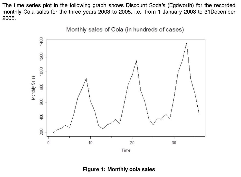
The time series plot in the following graph shows Discount Soda's (Egdworth) for the recorded monthly...
Fantastic news! We've Found the answer you've been seeking!
Question:
Transcribed Image Text:
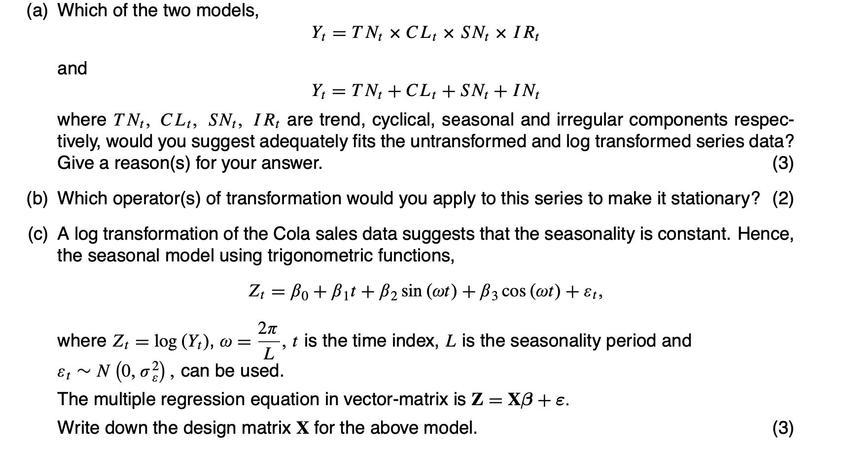
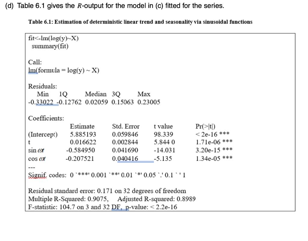
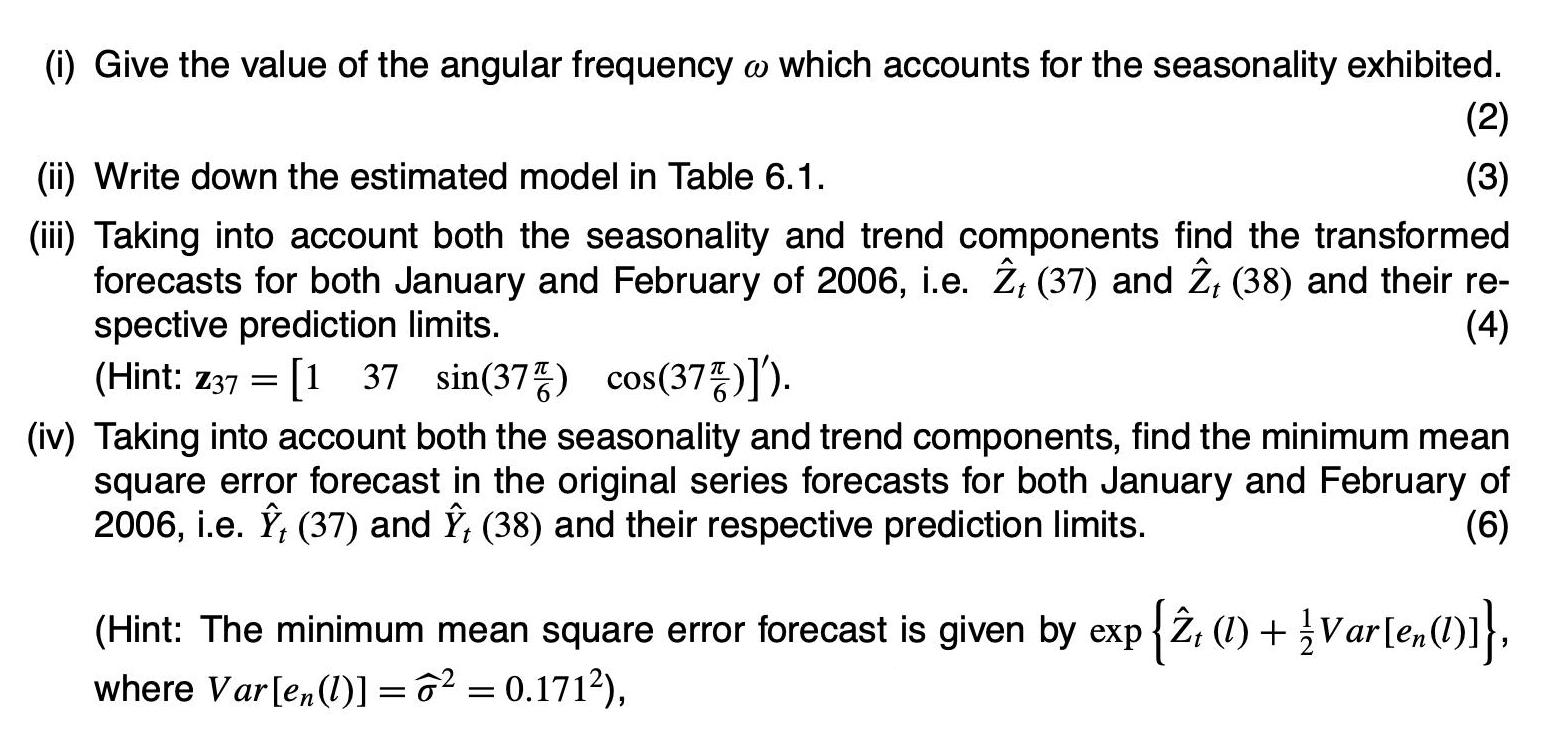
The time series plot in the following graph shows Discount Soda's (Egdworth) for the recorded monthly Cola sales for the three years 2003 to 2005, i.e. from 1 January 2003 to 31December 2005. Monthly sales of Cola (in hundreds of cases) 10 20 30 Time Figure 1: Monthly cola sales 000 0001 008 009 007 Monthly Sales (a) Which of the two models, Y; = TN; x CL; × SN; x IR; and Y; = TN; + CL; + SN; + IN, %3D where TN, CL, SN, IR, are trend, cyclical, seasonal and irregular components respec- tively, would you suggest adequately fits the untransformed and log transformed series data? Give a reason(s) for your answer. (3) (b) Which operator(s) of transformation would you apply to this series to make it stationary? (2) (c) A log transformation of the Cola sales data suggests that the seasonality is constant. Hence, the seasonal model using trigonometric functions, Z; = Bo + Bit +B2 sin (@t) + B3 cos (@t) + E1, %3D 2n t is the time index, L is the seasonality period and L where Z, log (Y;), w = Et ~ N (0, o?), can be used. The multiple regression equation in vector-matrix is Z = XB + e. Write down the design matrix X for the above model. (3) (d) Table 6.1 gives the R-output for the model in (c) fitted for the series. Table 6.1: Estimation of deterministic linear trend and seasonality via sinusoidal functions fit<-Im(log(y)~X) summary(fit) Call: Im(formula = log(y)~X) Residuals: Min 1Q Median 3Q Маx -0.33022 -0.12762 0.02059 0.15063 0.23005 Coefficients: Estimate Std. Error t value Pr(>It) < 2e-16 *** 1.71e-06 * ** 3.20e-15 *** 1.34e-05 *** (Intercept) 5.885193 0.059846 98.339 0.016622 0.002844 5.844 0 sin ot -0.584950 0.041690 -14.031 cos ot -0.207521 0.040416 -5.135 --- Signif. codes: 0 ***' 0.001 ***' 0.01 0.05 .'0.1 '1 Residual standard error: 0.171 on 32 degrees of freedom Multiple R-Squared: 0.9075, F-statistic: 104.7 on 3 and 32 DF, p-value: < 2.2e-16 Adjusted R-squared: 0.8989 (i) Give the value of the angular frequency o which accounts for the seasonality exhibited. (2) (ii) Write down the estimated model in Table 6.1. (3) (iii) Taking into account both the seasonality and trend components find the transformed forecasts for both January and February of 2006, i.e. Ż; (37) and 2; (38) and their re- spective prediction limits. (Hint: z373 [1 37 sin(37풍) cos(37등)]). (4) (iv) Taking into account both the seasonality and trend components, find the minimum mean square error forecast in the original series forecasts for both January and February of 2006, i.e. Î, (37) and Î, (38) and their respective prediction limits. (6) (Hint: The minimum mean square error forecast is given by exp {2, (1) +Var[e,1)]}, where Var[e,(1)1 = 62 = 0.1712), %3D The time series plot in the following graph shows Discount Soda's (Egdworth) for the recorded monthly Cola sales for the three years 2003 to 2005, i.e. from 1 January 2003 to 31December 2005. Monthly sales of Cola (in hundreds of cases) 10 20 30 Time Figure 1: Monthly cola sales 000 0001 008 009 007 Monthly Sales (a) Which of the two models, Y; = TN; x CL; × SN; x IR; and Y; = TN; + CL; + SN; + IN, %3D where TN, CL, SN, IR, are trend, cyclical, seasonal and irregular components respec- tively, would you suggest adequately fits the untransformed and log transformed series data? Give a reason(s) for your answer. (3) (b) Which operator(s) of transformation would you apply to this series to make it stationary? (2) (c) A log transformation of the Cola sales data suggests that the seasonality is constant. Hence, the seasonal model using trigonometric functions, Z; = Bo + Bit +B2 sin (@t) + B3 cos (@t) + E1, %3D 2n t is the time index, L is the seasonality period and L where Z, log (Y;), w = Et ~ N (0, o?), can be used. The multiple regression equation in vector-matrix is Z = XB + e. Write down the design matrix X for the above model. (3) (d) Table 6.1 gives the R-output for the model in (c) fitted for the series. Table 6.1: Estimation of deterministic linear trend and seasonality via sinusoidal functions fit<-Im(log(y)~X) summary(fit) Call: Im(formula = log(y)~X) Residuals: Min 1Q Median 3Q Маx -0.33022 -0.12762 0.02059 0.15063 0.23005 Coefficients: Estimate Std. Error t value Pr(>It) < 2e-16 *** 1.71e-06 * ** 3.20e-15 *** 1.34e-05 *** (Intercept) 5.885193 0.059846 98.339 0.016622 0.002844 5.844 0 sin ot -0.584950 0.041690 -14.031 cos ot -0.207521 0.040416 -5.135 --- Signif. codes: 0 ***' 0.001 ***' 0.01 0.05 .'0.1 '1 Residual standard error: 0.171 on 32 degrees of freedom Multiple R-Squared: 0.9075, F-statistic: 104.7 on 3 and 32 DF, p-value: < 2.2e-16 Adjusted R-squared: 0.8989 (i) Give the value of the angular frequency o which accounts for the seasonality exhibited. (2) (ii) Write down the estimated model in Table 6.1. (3) (iii) Taking into account both the seasonality and trend components find the transformed forecasts for both January and February of 2006, i.e. Ż; (37) and 2; (38) and their re- spective prediction limits. (Hint: z373 [1 37 sin(37풍) cos(37등)]). (4) (iv) Taking into account both the seasonality and trend components, find the minimum mean square error forecast in the original series forecasts for both January and February of 2006, i.e. Î, (37) and Î, (38) and their respective prediction limits. (6) (Hint: The minimum mean square error forecast is given by exp {2, (1) +Var[e,1)]}, where Var[e,(1)1 = 62 = 0.1712), %3D The time series plot in the following graph shows Discount Soda's (Egdworth) for the recorded monthly Cola sales for the three years 2003 to 2005, i.e. from 1 January 2003 to 31December 2005. Monthly sales of Cola (in hundreds of cases) 10 20 30 Time Figure 1: Monthly cola sales 000 0001 008 009 007 Monthly Sales (a) Which of the two models, Y; = TN; x CL; × SN; x IR; and Y; = TN; + CL; + SN; + IN, %3D where TN, CL, SN, IR, are trend, cyclical, seasonal and irregular components respec- tively, would you suggest adequately fits the untransformed and log transformed series data? Give a reason(s) for your answer. (3) (b) Which operator(s) of transformation would you apply to this series to make it stationary? (2) (c) A log transformation of the Cola sales data suggests that the seasonality is constant. Hence, the seasonal model using trigonometric functions, Z; = Bo + Bit +B2 sin (@t) + B3 cos (@t) + E1, %3D 2n t is the time index, L is the seasonality period and L where Z, log (Y;), w = Et ~ N (0, o?), can be used. The multiple regression equation in vector-matrix is Z = XB + e. Write down the design matrix X for the above model. (3) (d) Table 6.1 gives the R-output for the model in (c) fitted for the series. Table 6.1: Estimation of deterministic linear trend and seasonality via sinusoidal functions fit<-Im(log(y)~X) summary(fit) Call: Im(formula = log(y)~X) Residuals: Min 1Q Median 3Q Маx -0.33022 -0.12762 0.02059 0.15063 0.23005 Coefficients: Estimate Std. Error t value Pr(>It) < 2e-16 *** 1.71e-06 * ** 3.20e-15 *** 1.34e-05 *** (Intercept) 5.885193 0.059846 98.339 0.016622 0.002844 5.844 0 sin ot -0.584950 0.041690 -14.031 cos ot -0.207521 0.040416 -5.135 --- Signif. codes: 0 ***' 0.001 ***' 0.01 0.05 .'0.1 '1 Residual standard error: 0.171 on 32 degrees of freedom Multiple R-Squared: 0.9075, F-statistic: 104.7 on 3 and 32 DF, p-value: < 2.2e-16 Adjusted R-squared: 0.8989 (i) Give the value of the angular frequency o which accounts for the seasonality exhibited. (2) (ii) Write down the estimated model in Table 6.1. (3) (iii) Taking into account both the seasonality and trend components find the transformed forecasts for both January and February of 2006, i.e. Ż; (37) and 2; (38) and their re- spective prediction limits. (Hint: z373 [1 37 sin(37풍) cos(37등)]). (4) (iv) Taking into account both the seasonality and trend components, find the minimum mean square error forecast in the original series forecasts for both January and February of 2006, i.e. Î, (37) and Î, (38) and their respective prediction limits. (6) (Hint: The minimum mean square error forecast is given by exp {2, (1) +Var[e,1)]}, where Var[e,(1)1 = 62 = 0.1712), %3D The time series plot in the following graph shows Discount Soda's (Egdworth) for the recorded monthly Cola sales for the three years 2003 to 2005, i.e. from 1 January 2003 to 31December 2005. Monthly sales of Cola (in hundreds of cases) 10 20 30 Time Figure 1: Monthly cola sales 000 0001 008 009 007 Monthly Sales (a) Which of the two models, Y; = TN; x CL; × SN; x IR; and Y; = TN; + CL; + SN; + IN, %3D where TN, CL, SN, IR, are trend, cyclical, seasonal and irregular components respec- tively, would you suggest adequately fits the untransformed and log transformed series data? Give a reason(s) for your answer. (3) (b) Which operator(s) of transformation would you apply to this series to make it stationary? (2) (c) A log transformation of the Cola sales data suggests that the seasonality is constant. Hence, the seasonal model using trigonometric functions, Z; = Bo + Bit +B2 sin (@t) + B3 cos (@t) + E1, %3D 2n t is the time index, L is the seasonality period and L where Z, log (Y;), w = Et ~ N (0, o?), can be used. The multiple regression equation in vector-matrix is Z = XB + e. Write down the design matrix X for the above model. (3) (d) Table 6.1 gives the R-output for the model in (c) fitted for the series. Table 6.1: Estimation of deterministic linear trend and seasonality via sinusoidal functions fit<-Im(log(y)~X) summary(fit) Call: Im(formula = log(y)~X) Residuals: Min 1Q Median 3Q Маx -0.33022 -0.12762 0.02059 0.15063 0.23005 Coefficients: Estimate Std. Error t value Pr(>It) < 2e-16 *** 1.71e-06 * ** 3.20e-15 *** 1.34e-05 *** (Intercept) 5.885193 0.059846 98.339 0.016622 0.002844 5.844 0 sin ot -0.584950 0.041690 -14.031 cos ot -0.207521 0.040416 -5.135 --- Signif. codes: 0 ***' 0.001 ***' 0.01 0.05 .'0.1 '1 Residual standard error: 0.171 on 32 degrees of freedom Multiple R-Squared: 0.9075, F-statistic: 104.7 on 3 and 32 DF, p-value: < 2.2e-16 Adjusted R-squared: 0.8989 (i) Give the value of the angular frequency o which accounts for the seasonality exhibited. (2) (ii) Write down the estimated model in Table 6.1. (3) (iii) Taking into account both the seasonality and trend components find the transformed forecasts for both January and February of 2006, i.e. Ż; (37) and 2; (38) and their re- spective prediction limits. (Hint: z373 [1 37 sin(37풍) cos(37등)]). (4) (iv) Taking into account both the seasonality and trend components, find the minimum mean square error forecast in the original series forecasts for both January and February of 2006, i.e. Î, (37) and Î, (38) and their respective prediction limits. (6) (Hint: The minimum mean square error forecast is given by exp {2, (1) +Var[e,1)]}, where Var[e,(1)1 = 62 = 0.1712), %3D The time series plot in the following graph shows Discount Soda's (Egdworth) for the recorded monthly Cola sales for the three years 2003 to 2005, i.e. from 1 January 2003 to 31December 2005. Monthly sales of Cola (in hundreds of cases) 10 20 30 Time Figure 1: Monthly cola sales 000 0001 008 009 007 Monthly Sales (a) Which of the two models, Y; = TN; x CL; × SN; x IR; and Y; = TN; + CL; + SN; + IN, %3D where TN, CL, SN, IR, are trend, cyclical, seasonal and irregular components respec- tively, would you suggest adequately fits the untransformed and log transformed series data? Give a reason(s) for your answer. (3) (b) Which operator(s) of transformation would you apply to this series to make it stationary? (2) (c) A log transformation of the Cola sales data suggests that the seasonality is constant. Hence, the seasonal model using trigonometric functions, Z; = Bo + Bit +B2 sin (@t) + B3 cos (@t) + E1, %3D 2n t is the time index, L is the seasonality period and L where Z, log (Y;), w = Et ~ N (0, o?), can be used. The multiple regression equation in vector-matrix is Z = XB + e. Write down the design matrix X for the above model. (3) (d) Table 6.1 gives the R-output for the model in (c) fitted for the series. Table 6.1: Estimation of deterministic linear trend and seasonality via sinusoidal functions fit<-Im(log(y)~X) summary(fit) Call: Im(formula = log(y)~X) Residuals: Min 1Q Median 3Q Маx -0.33022 -0.12762 0.02059 0.15063 0.23005 Coefficients: Estimate Std. Error t value Pr(>It) < 2e-16 *** 1.71e-06 * ** 3.20e-15 *** 1.34e-05 *** (Intercept) 5.885193 0.059846 98.339 0.016622 0.002844 5.844 0 sin ot -0.584950 0.041690 -14.031 cos ot -0.207521 0.040416 -5.135 --- Signif. codes: 0 ***' 0.001 ***' 0.01 0.05 .'0.1 '1 Residual standard error: 0.171 on 32 degrees of freedom Multiple R-Squared: 0.9075, F-statistic: 104.7 on 3 and 32 DF, p-value: < 2.2e-16 Adjusted R-squared: 0.8989 (i) Give the value of the angular frequency o which accounts for the seasonality exhibited. (2) (ii) Write down the estimated model in Table 6.1. (3) (iii) Taking into account both the seasonality and trend components find the transformed forecasts for both January and February of 2006, i.e. Ż; (37) and 2; (38) and their re- spective prediction limits. (Hint: z373 [1 37 sin(37풍) cos(37등)]). (4) (iv) Taking into account both the seasonality and trend components, find the minimum mean square error forecast in the original series forecasts for both January and February of 2006, i.e. Î, (37) and Î, (38) and their respective prediction limits. (6) (Hint: The minimum mean square error forecast is given by exp {2, (1) +Var[e,1)]}, where Var[e,(1)1 = 62 = 0.1712), %3D The time series plot in the following graph shows Discount Soda's (Egdworth) for the recorded monthly Cola sales for the three years 2003 to 2005, i.e. from 1 January 2003 to 31December 2005. Monthly sales of Cola (in hundreds of cases) 10 20 30 Time Figure 1: Monthly cola sales 000 0001 008 009 007 Monthly Sales (a) Which of the two models, Y; = TN; x CL; × SN; x IR; and Y; = TN; + CL; + SN; + IN, %3D where TN, CL, SN, IR, are trend, cyclical, seasonal and irregular components respec- tively, would you suggest adequately fits the untransformed and log transformed series data? Give a reason(s) for your answer. (3) (b) Which operator(s) of transformation would you apply to this series to make it stationary? (2) (c) A log transformation of the Cola sales data suggests that the seasonality is constant. Hence, the seasonal model using trigonometric functions, Z; = Bo + Bit +B2 sin (@t) + B3 cos (@t) + E1, %3D 2n t is the time index, L is the seasonality period and L where Z, log (Y;), w = Et ~ N (0, o?), can be used. The multiple regression equation in vector-matrix is Z = XB + e. Write down the design matrix X for the above model. (3) (d) Table 6.1 gives the R-output for the model in (c) fitted for the series. Table 6.1: Estimation of deterministic linear trend and seasonality via sinusoidal functions fit<-Im(log(y)~X) summary(fit) Call: Im(formula = log(y)~X) Residuals: Min 1Q Median 3Q Маx -0.33022 -0.12762 0.02059 0.15063 0.23005 Coefficients: Estimate Std. Error t value Pr(>It) < 2e-16 *** 1.71e-06 * ** 3.20e-15 *** 1.34e-05 *** (Intercept) 5.885193 0.059846 98.339 0.016622 0.002844 5.844 0 sin ot -0.584950 0.041690 -14.031 cos ot -0.207521 0.040416 -5.135 --- Signif. codes: 0 ***' 0.001 ***' 0.01 0.05 .'0.1 '1 Residual standard error: 0.171 on 32 degrees of freedom Multiple R-Squared: 0.9075, F-statistic: 104.7 on 3 and 32 DF, p-value: < 2.2e-16 Adjusted R-squared: 0.8989 (i) Give the value of the angular frequency o which accounts for the seasonality exhibited. (2) (ii) Write down the estimated model in Table 6.1. (3) (iii) Taking into account both the seasonality and trend components find the transformed forecasts for both January and February of 2006, i.e. Ż; (37) and 2; (38) and their re- spective prediction limits. (Hint: z373 [1 37 sin(37풍) cos(37등)]). (4) (iv) Taking into account both the seasonality and trend components, find the minimum mean square error forecast in the original series forecasts for both January and February of 2006, i.e. Î, (37) and Î, (38) and their respective prediction limits. (6) (Hint: The minimum mean square error forecast is given by exp {2, (1) +Var[e,1)]}, where Var[e,(1)1 = 62 = 0.1712), %3D The time series plot in the following graph shows Discount Soda's (Egdworth) for the recorded monthly Cola sales for the three years 2003 to 2005, i.e. from 1 January 2003 to 31December 2005. Monthly sales of Cola (in hundreds of cases) 10 20 30 Time Figure 1: Monthly cola sales 000 0001 008 009 007 Monthly Sales (a) Which of the two models, Y; = TN; x CL; × SN; x IR; and Y; = TN; + CL; + SN; + IN, %3D where TN, CL, SN, IR, are trend, cyclical, seasonal and irregular components respec- tively, would you suggest adequately fits the untransformed and log transformed series data? Give a reason(s) for your answer. (3) (b) Which operator(s) of transformation would you apply to this series to make it stationary? (2) (c) A log transformation of the Cola sales data suggests that the seasonality is constant. Hence, the seasonal model using trigonometric functions, Z; = Bo + Bit +B2 sin (@t) + B3 cos (@t) + E1, %3D 2n t is the time index, L is the seasonality period and L where Z, log (Y;), w = Et ~ N (0, o?), can be used. The multiple regression equation in vector-matrix is Z = XB + e. Write down the design matrix X for the above model. (3) (d) Table 6.1 gives the R-output for the model in (c) fitted for the series. Table 6.1: Estimation of deterministic linear trend and seasonality via sinusoidal functions fit<-Im(log(y)~X) summary(fit) Call: Im(formula = log(y)~X) Residuals: Min 1Q Median 3Q Маx -0.33022 -0.12762 0.02059 0.15063 0.23005 Coefficients: Estimate Std. Error t value Pr(>It) < 2e-16 *** 1.71e-06 * ** 3.20e-15 *** 1.34e-05 *** (Intercept) 5.885193 0.059846 98.339 0.016622 0.002844 5.844 0 sin ot -0.584950 0.041690 -14.031 cos ot -0.207521 0.040416 -5.135 --- Signif. codes: 0 ***' 0.001 ***' 0.01 0.05 .'0.1 '1 Residual standard error: 0.171 on 32 degrees of freedom Multiple R-Squared: 0.9075, F-statistic: 104.7 on 3 and 32 DF, p-value: < 2.2e-16 Adjusted R-squared: 0.8989 (i) Give the value of the angular frequency o which accounts for the seasonality exhibited. (2) (ii) Write down the estimated model in Table 6.1. (3) (iii) Taking into account both the seasonality and trend components find the transformed forecasts for both January and February of 2006, i.e. Ż; (37) and 2; (38) and their re- spective prediction limits. (Hint: z373 [1 37 sin(37풍) cos(37등)]). (4) (iv) Taking into account both the seasonality and trend components, find the minimum mean square error forecast in the original series forecasts for both January and February of 2006, i.e. Î, (37) and Î, (38) and their respective prediction limits. (6) (Hint: The minimum mean square error forecast is given by exp {2, (1) +Var[e,1)]}, where Var[e,(1)1 = 62 = 0.1712), %3D The time series plot in the following graph shows Discount Soda's (Egdworth) for the recorded monthly Cola sales for the three years 2003 to 2005, i.e. from 1 January 2003 to 31December 2005. Monthly sales of Cola (in hundreds of cases) 10 20 30 Time Figure 1: Monthly cola sales 000 0001 008 009 007 Monthly Sales (a) Which of the two models, Y; = TN; x CL; × SN; x IR; and Y; = TN; + CL; + SN; + IN, %3D where TN, CL, SN, IR, are trend, cyclical, seasonal and irregular components respec- tively, would you suggest adequately fits the untransformed and log transformed series data? Give a reason(s) for your answer. (3) (b) Which operator(s) of transformation would you apply to this series to make it stationary? (2) (c) A log transformation of the Cola sales data suggests that the seasonality is constant. Hence, the seasonal model using trigonometric functions, Z; = Bo + Bit +B2 sin (@t) + B3 cos (@t) + E1, %3D 2n t is the time index, L is the seasonality period and L where Z, log (Y;), w = Et ~ N (0, o?), can be used. The multiple regression equation in vector-matrix is Z = XB + e. Write down the design matrix X for the above model. (3) (d) Table 6.1 gives the R-output for the model in (c) fitted for the series. Table 6.1: Estimation of deterministic linear trend and seasonality via sinusoidal functions fit<-Im(log(y)~X) summary(fit) Call: Im(formula = log(y)~X) Residuals: Min 1Q Median 3Q Маx -0.33022 -0.12762 0.02059 0.15063 0.23005 Coefficients: Estimate Std. Error t value Pr(>It) < 2e-16 *** 1.71e-06 * ** 3.20e-15 *** 1.34e-05 *** (Intercept) 5.885193 0.059846 98.339 0.016622 0.002844 5.844 0 sin ot -0.584950 0.041690 -14.031 cos ot -0.207521 0.040416 -5.135 --- Signif. codes: 0 ***' 0.001 ***' 0.01 0.05 .'0.1 '1 Residual standard error: 0.171 on 32 degrees of freedom Multiple R-Squared: 0.9075, F-statistic: 104.7 on 3 and 32 DF, p-value: < 2.2e-16 Adjusted R-squared: 0.8989 (i) Give the value of the angular frequency o which accounts for the seasonality exhibited. (2) (ii) Write down the estimated model in Table 6.1. (3) (iii) Taking into account both the seasonality and trend components find the transformed forecasts for both January and February of 2006, i.e. Ż; (37) and 2; (38) and their re- spective prediction limits. (Hint: z373 [1 37 sin(37풍) cos(37등)]). (4) (iv) Taking into account both the seasonality and trend components, find the minimum mean square error forecast in the original series forecasts for both January and February of 2006, i.e. Î, (37) and Î, (38) and their respective prediction limits. (6) (Hint: The minimum mean square error forecast is given by exp {2, (1) +Var[e,1)]}, where Var[e,(1)1 = 62 = 0.1712), %3D
Expert Answer:
Answer rating: 100% (QA)
Generally two types of models are used in time series forecasting 1 Additive model such as ... View the full answer

Related Book For 

Business Statistics
ISBN: 978-0321925831
3rd edition
Authors: Norean Sharpe, Richard Veaux, Paul Velleman
Posted Date:
Students also viewed these biology questions
-
Following is the time series plot for the monthly U.S. Unemployment rate (%) from January 2003 to June 2013. These data have been seasonally adjusted (meaning that the seasonal component has already...
-
The dotted line in the following graph shows levels of glucose in a culture of wild-type E, coli grown in medium that initially contains both glucose and lactose. The solid line shows levels of...
-
Figure Q28.19 shows a series combination of three lightbulbs, all rated at 120 V with power ratings of 60 W, 75 W, and 200 W. Why is the 60-W lamp the brightest and the 200-W lamp the dimmest? Which...
-
3) Sauseda Corporation has two operating divisions-an Inland Division and a Coast Division. The company's Customer Service Department provides services to both divisions. The variable costs of the...
-
Immigration reform has focused on dividing illegal immigrants into two groups: long-term and short-term. In a random sample of 958 construction workers from the Northeast, 66 are illegal short-term...
-
Each of two identical objects carries a net charge. The objects are made from conducting material. One object is attracted to a positively charged ebonite rod, and the other is repelled by the rod....
-
Apply ridge regression to the Hald cement data in Table B.21. a. Use the ridge trace to select an appropriate value of \(k\). Is the final model a good one? b. How much inflation in the residual sum...
-
During the first-year audit of Jones Wholesale Stationery, you observe that commissions amount to almost 25 percent of total sales, which is somewhat higher than in previous years. Further...
-
The table below shows information about the action figures available in a toy shop. Syed picks one at random for his niece. a) Work out P(shield female) as a fraction in its simplest form. b) Is the...
-
In 2008, Wayne Singleton and his eight-year-old son, Jaron, were traveling on a bus for a school field trip to Six Flags. Wayne fell asleep on the way, and while he was asleep, the bus became...
-
August 1. Invested $30,000 cash and equipment valued at $10,000 in the business 2. Purchased supplies on account for $2,000. 3. Paid office rent of $1,200 for a year. 5. Completed audit of financial...
-
You and your partner own Gaia's Organic Grocery: You buy your romaine lettuce from Naturally Yours Garden Farm. Unknown to you, Naturally Yours' romaine has been infected by a microscopic parasite...
-
12. Due to the popularity of the ice cream, Ben and James have decided to expand their team and lease more workspace. The new space needs to be renovated and Ben has entered into a contract with...
-
Learning Activity 8: Slander or Libel Let's return to the four examples given at the beginning of this lesson. 1. Your ex-partner says you were a clumsy dancer and boring. Were you slandered? What...
-
The following salaried employees of Mountain Stone Brewery in Fort Collins, Colorado, are paid semimonthly. Some employees have union dues or garnishments deducted from their pay. You do not need to...
-
Spenser Manufacturing Ltd.'s prepaid rent balance was $12,500 at December 31, 2021 and $8,400 at December 31, 2020. On its income statements Spenser reported Rent expense of $6,000 for 2021, and...
-
mRNA PART B. Answer the following questions on your paper: 1. What is the first step of protein synthesis? 2. What is the second step of protein synthesis? 3. Where does the first step of protein...
-
Find the image of x = k = const under w = 1/z. Use formulas similar to those in Example 1. y| y = 0 -21 -2 -1 -1, /1 12 T -1 -1 y= -2 x =0
-
GfK Roper surveyed people worldwide asking them how important is acquiring wealth to you. Of 1535 respondents in India, 1168 said that it was of more than average importance. In the United States of...
-
In Chapter 17, Exercise 36 we found a model for HDI (the UNs Human Development Index) from 7 socio-economic variables for 96 countries. Using software that provides regression diagnostics (leverage...
-
In the early days of the iPod, MacInTouch (www.macintouch.com/reliability/ipod failures.html) surveyed readers about reliability. Of the 8926 iPods owned at that time, 7510 were problem-free while...
-
Brown India Limited manufactures office tables. Normal capacity of the factory is 60,000 tables per annum. Following are the cost and inventory details for the year 200506. Required: Carry out the...
-
Usha Corporation Ltd. sought the advice of an investment advisor for deployment of surplus funds of around Rs. 45 lakh in the stock market. The advisor advised to invest in Bhonsle India Ltd. and...
-
Ram Lakhan Company Ltd. produces one unit of product B by using one unit of raw material A. During 200506 A costed the company 4,200. Conversion cost was 850. As on 31st March 2006, being the...

Study smarter with the SolutionInn App