Use Mathematica to solve the system of equations (1.1.1) and (1.1.4) (1.1.6) for two coupled wells, for
Question:
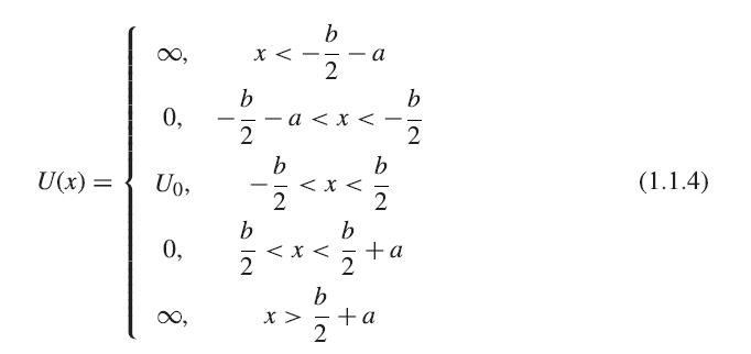
Use Mathematica to solve the system of equations (1.1.1) and (1.1.4)– (1.1.6) for two coupled wells, for the case 2mU0/h̄2 = 20, a = 1, and b = 0.1. The calculation can be greatly simplified by assuming that the solution has the form ψ1(x) = A1 sin(Kx) + B1 cos(Kx), ψ2(x) = A2(eκx ± e−κx), and ψ3(x) = ±ψ1(−x), where the + and − signs correspond to the symmetric and antisymmetric solutions, respectively. Since the overall amplitude of the wave doesn’t matter, you can set A1 = 1. In this case, there are four unknowns B1, A2, K, and κ, and four equations, namely three independent boundary conditions and (1.1.1) in the barrier region, which gives κ in terms of K. B1 and A2 can be easily eliminated algebraically. You are left with a complicated equation for K; you can find the roots by first graphing both sides as functions of K to see approximately where the two sides are equal, and then using the Mathematica function FindRoot to get an exact value for K.
Plot the energy splitting of the two lowest energy states (the symmetric and antisymmetric combinations of the ground state) for various choices of the barrier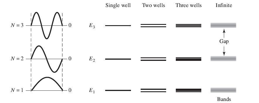
thickness b. In the limit of infinite separation, they should have the same energy. Note that in the limit b → 0, the symmetric and antisymmetric solutions of the two wells simply become the N = 1 and N = 2 solutions for a single square well. Plot the wave function for a typical value of b. Since the function has three parts, you will have to use the Mathematica function Show to combine the three function plots.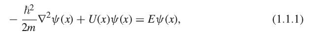

Step by Step Answer:
According to the prescription of the text we assume that the solutions in the two regions take the f...View the full answer