Consider again Example 2. 2. The result in (2.53) suggests that (mathbb{E} widehat{boldsymbol{beta}} ightarrow beta_{p}) as

Consider again Example 2.

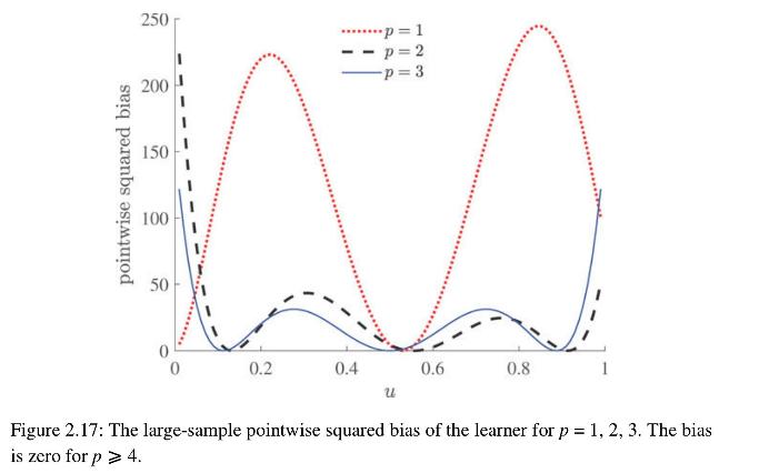
2. The result in (2.53) suggests that \(\mathbb{E} \widehat{\boldsymbol{\beta}} \rightarrow \beta_{p}\) as \(n \rightarrow \infty\), where \(\beta_{p}\) is the solution in the class \(\mathscr{G}_{p}\) given in (2.18). Thus, the large-sample approximation of the pointwise bias of the learner \(g_{\mathscr{T}}^{\mathscr{G}_{p}}(\boldsymbol{x})=\boldsymbol{x}^{\top} \widehat{\boldsymbol{\beta}}\) at \(\boldsymbol{x}=\left[1, \ldots, u^{p-1}\right]^{\top}\) is

\[ \mathbb{E} g_{\mathscr{T}}^{\mathscr{C}_{p}}(\boldsymbol{x})-g^{*}(\boldsymbol{x}) \simeq\left[1, \ldots, u^{p-1}\right] \boldsymbol{\beta}_{p}-\left[1, u, u^{2}, u^{3}\right] \boldsymbol{\beta}^{3}, \quad n \rightarrow \infty \]

Use Python to reproduce Figure 2.

17, which shows the (large-sample) pointwise squared bias of the learner for \(p \in\{1,2,3\}\). Note how the bias is larger near the endpoints \(u=0\) and \(u=1\). Explain why the areas under the curves correspond to the approximation errors.

Plot this large-sample approximation of the expected statistical error and compare it with the outcome of the statistical error.

Transcribed Image Text:

pointwise squared bias 250 200 150 100 50 - p=2 -p=3. 0.2 0.4 0.6 0.8 Figure 2.17: The large-sample pointwise squared bias of the learner for p = 1, 2, 3. The bias is zero for p > 4.