Follow the analysis of Example 5.7 to discriminate between the five files with EEG data. Apply a similar analysis to discriminate between the data in the files EEGsetB.CSV, EEGsetC.CSv and EEGsetE.csv. Select the best way to classify the five files between seizure and healthy individuals and compare different discrimination methods using the five files, A to E.

Data From Example 5.7:

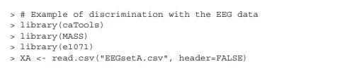
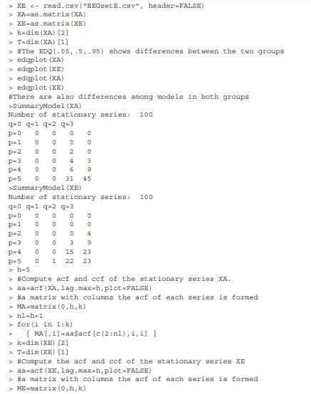
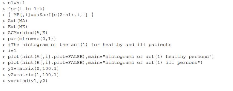
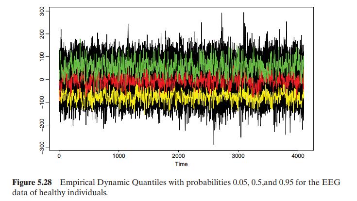
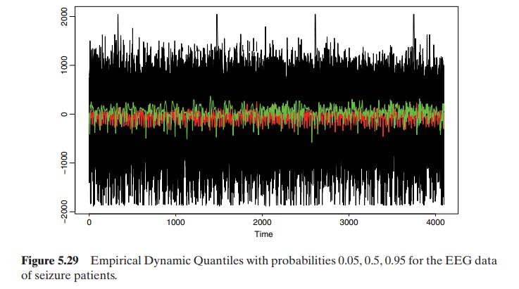
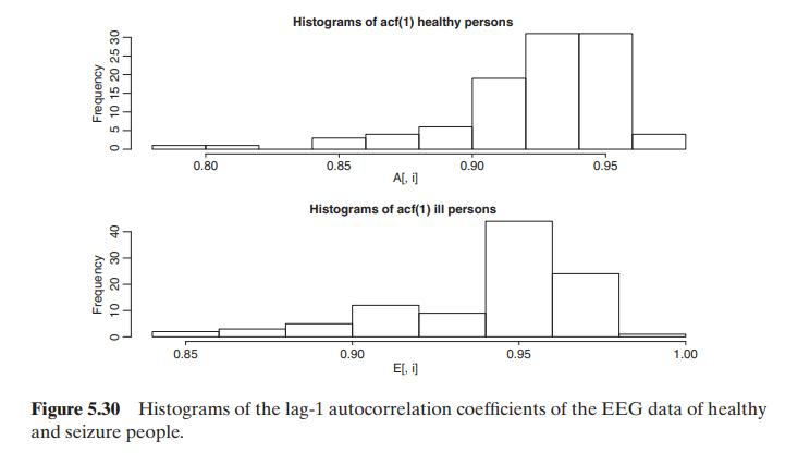
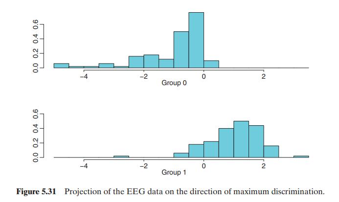
We consider the series of electroencephalograms (EEG) studied by Andrzejak et al. (2001) and Maharaj and Alonso (2007). An EEG is a recording of the electrical activity of the brain. We have 200 time series of individuals with \(T=4096\) observations of EEG. The first 100 series, type A, correspond to healthy volunteers whereas the second 100 series, type E, consist of EEG recordings during seizure activity of patients. Figures 5.28 and 5.29 show the time series plots along with three EDQ (prob \(=0.01,0.5,0.95\) ) of Chapter 2. From the plots, we see that the EEG series for seizure patients, type E, have much more extreme values than those of healthy individuals, type A. This feature can be useful for discrimination. We fit ARIMA models to the series in both groups using the command SummaryModel and found that series of type A mostly follow \((76 \%)\) an ARMA( 5,3 ) or ARMA \((5,2)\) model, whereas series in type E mostly follow ( \(55 \%\) ) other ARMA models. As an illustration, in this example we use the first 5 autocorrelation coefficients to classify the data. Figure 5.30 show that the histograms of the lag-1 ACF for both groups are different, but the differences are small. We apply the LDF and logistic regression (LG) to the EEG data. These two methods are first applied to all the data, then they are estimated in a training sample that includes \(65 \%\) of the data and evaluated in the test sample with the remaining \(35 \%\) of the data. Figure 5.31 shows the projection of the data in the direction of maximum discrimination computed with LDF. The estimated model for LR has all coefficients statistically significant and is shown in the output. With all the data, the discrimination errors are 9 for LDF and \(2.5 \%\) for LR. However, when the split sample LDF has \(8 \%\) error in the training sample and \(16 \%\) in the test sample, whereas LR has \(3 \%\) in the training sample and \(33 \%\) in the test sample. These results suggest some overfitting in the LR. To compare the two methods with just one sample may be misleading and it is useful to replicate the analysis with several splits in training and test data. With 50 splits and using the program discrim that carries out all the analysis, the average results for LDF is 8% in sample and 13% in the out of sample and for LR 3% in sample and 13% out of sample. Thus, both methods perform similarly in this example.

R commands and analysis of EEG data 

Transcribed Image Text:

> # Example of discrimination with the EEG data > library(caTools) > library (MASS) > library(e1071) > XA