Question: For our model presented in Example 2, test the hypotheses where (beta_{1}) is the slope coefficient for the explanatory variable age, and (beta_{2}) is the

For our model presented in Example 2, test the hypotheses

Ho: B = 0 VS. H: B0 Ho: B = 0 VS.
where $\beta_{1}$ is the slope coefficient for the explanatory variable age, and $\beta_{2}$ is the slope coefficient for the explanatory variable saturated fat.
Approach We will use Minitab to determine the $P$-values for each explanatory variable. If the $P$-value is less than the level of significance, we reject the null hypothesis and conclude that the slope coefficient is different from zero.

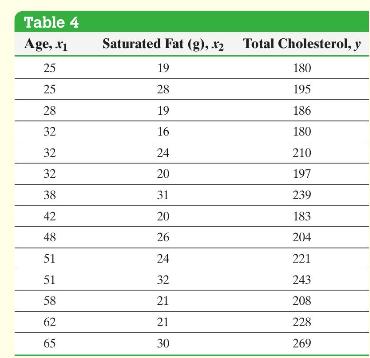
Data from Example 2

Use the data in Table 4.

Find the least-squares regression equation $\hat{y}=b_{0}+b_{1} x_{1}+b_{2} x_{2}$, where $x_{1}$ represents the patient's age, $x_{2}$ represents the patient's daily consumption of saturated fat, and $y$ represents the patient's total cholesterol.

Draw residual plots and a boxplot of the residuals to assess the adequacy of the model.

Enter the data into Minitab to obtain the least-squares regression equation and to draw the residual plots and boxplot of the residuals. The steps for determining the multiple regression equation and residual plots using Minitab, Excel, and StatCrunch are given in the Technology Step-by-Step.

H: B 0

Ho: B = 0 VS. H: B0 Ho: B = 0 VS. H: B 0

Step by Step Solution

★★★★★

3.45 Rating (155 Votes )

There are 3 Steps involved in it

1 Expert Approved Answer

Step: 1 Unlock

Looking again to the output in Figure 15 we see that the test statistic for the explana... View full answer

Question Has Been Solved by an Expert!

Get step-by-step solutions from verified subject matter experts

Step: 2 Unlock

Step: 3 Unlock

Students Have Also Explored These Related Statistics Informed Decisions Using Data Questions!

Verify the normality requirement for the HDL data analyzed in Example 3. Approach We will use Minitab to obtain the residuals and draw the normal probability plot. Data from Example 3 We presented...

Use statistical software to perform Tukey's test to determine which pairwise means differ for the data presented in Example 3 using a familywise error rate of $\alpha=0.05$. Approach We will use...

CANMNMM January of this year. (a) Each item will be held in a record. Describe all the data structures that must refer to these records to implement the required functionality. Describe all the...

Create charts to better understand data sets. For cross-sectional data, use a scatter chart. For time series data, use a line chart. Linear y = a + bx Logarithmic y = ln(x) Polynomial (2nd order) y =...

Location Income ($1,000) Urban 27 Rural 25 Suburban 25 Suburban 26 Rural 30 Urban 29 Rural 33 Urban 30 Suburban 32 Urban 34 Urban 35 Urban 40 Rural 30 Rural 33 Urban 42 Suburban 32 Urban 43 Urban 43...

Instructor: Basu Dipanker Course: MAT-240-Q6622-16EW6 Assignment: 6-2 MyStatLab: Module Six Problem Set 1. Determine whether the scatter diagram indicates that a linear relation may exist between the...

Exercise 16.5 shows that given the three observations on binary choice with $y_{1}=1, y_{2}=1, y_{3}=0$ the maximum likelihood estimator of the logit model $P(y=1)=\Lambda\left(\gamma_{1} ight)$...

Set Student Name: 1. Describe the relationship between two variables that have a correlation coefficient value: a. Near -1 b. Near 0 c. Near 1 2. Data was collected where a weightlifter was asked to...

1. Suppose a least-squares regression line is given by y = 4.302x 3.293. What is the mean value of the response variable if x = 20? y 20 = (Round to one decimal place as needed.) 2. In the...

** You can use EXCEL or any other software. ** You need to include your printout in your submissions. The layout and format of the paper should include the following sections: Title page, Abstract,...

The adjusted trial balance of A Plus Events Piano Tuning Service, Inc., at fiscal year end October 31, 2012, follows. Requirements 1. Prepare A Plus's 2012 income statement. 2. Prepare the statement...

5. It is given a pyramid ABCD: A(3,5.1,4), B(5,10,1,4), C(8,7,1,4), D(4,7,1.8). Compute the volume and the height passing through the vertex D.

Use the method of steepest descent to find the maximum of the following objective function: U ( x , y ) = - ( N 1 0 + 1 ) ( x + N ) x - ( N 4 0 + 1 ) ( y - N ) y + x y 2 0 - N Start the search at the...

What is technology risk? What is the difference between economies of scale and economies of scope? How can these economies create benefits for an FI? How can these economies prove harmful to an FI?...

f(x) = 2 cos x (a) Find the zeros of f on the interval [-2, 4]. (b) Graph f(x) = 2 cos x on the interval [-2, 4]. (c) Solve f(x) = -3 on the interval [-2, 4]. What points are on the graph of f? Label...

f(x) = 4 tan x (a) Solve f(x) = -4. (b) For what values of x is f(x)

f(x) = cot x (a) Solve f(x) = -3. (b) For what values of x is f(x) > - 3 on the interval (0, )?

Define the System Development Life Cycle ( SDLC ) . How many phases are there in the SDLC ? Discuss each of them

9 . You have a bond with 5 years maturity and 6 % coupon ( interest ) rate. A coupon is paid annually. Its face value is $ 1 0 0 0 . If the bond is priced at $ 9 8 0 , how much is the Yield to...

1.Briefly describe the agency problem that exists between owners and lenders. How do lenders cause firms to incur agency costs to resolve this problem? 2. Please provide 3 references?