Example 12.4 described a study in which salmon were introduced to 12 streams with and without brook trout to investigate the effect of brook trout on salmon survival. Is this an experimental study or an observational study? Explain the basis for your reasoning.

Data from example  12.4

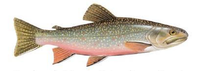
One of the greatest threats to biodiversity is the introduction of alien species from outside their natural range. These introduced species often have fewer predators or parasites in the new area, so they can increase in numbers and outcompete native species. Sometimes these species are introduced accidentally, but often they are introduced intentionally by humans. The brook trout, for example, is a species native to eastern North America that has been introduced into streams in the West for sport fishing. Biologists followed the survivorship of a native species, chinook salmon, in a series of 12 streams that either had brook trout introduced or did not (Levin et al. 2002). Their goal was to determine whether the presence of brook trout affected the survivorship of the salmon. In each stream, they released a number of tagged juvenile chinook and then recorded whether or not each chinook survived over one year. Table 12.4- summarizes the data.

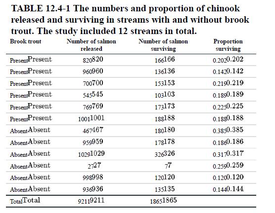
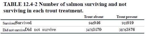
In all, 9211 salmon were released, of which 1865 survived and 7346 did not. A quick tally of the fish numbers by treatment yields the 2×2 table shown in Table 12.4-2.

We would like to test whether the proportion of salmon surviving differed between trout treatments. What method shall we use? It is tempting to carry out a χ² contingency test of association between treatment and survival.

The problem with using the contingency test approach is that individual salmon are not a random sample. Rather, salmon are grouped by the streams in which they were released. If there is any inherent difference between the streams in the probability of survival, over and above any effects of brook trout, then two salmon from the same stream are likely to be more similar in their survival than two salmon picked at random. In this case, salmon from the same stream are not independent. To lump all the salmon together and analyze with a contingency test is to commit the sin of pseudoreplication (see Interleaf 2).

The key to solving the problem lies in recognizing that the stream is the independently sampled unit, not the salmon, and there are only 12 streams —six per treatment. As a result, the fates of all the salmon within a stream must be summarized by a single measurement for analysis—namely, the proportion of salmon surviving (given in the last column of Table 12.4-2).

This changes the data type, because we are no longer comparing frequencies in categories, but rather differences in the means of a numerical variable. A two-sample test of the difference between the means is therefore required.

Let’s label the streams with trout present as group  and the streams without trout as group 2. The null and alternative hypotheses are as follows:

H₀: The mean proportion of chinook surviving is the same in streams with and without brook trout (μ₁=μ₂). H_A: The mean proportion of chinook surviving is different between streams with and without brook trout (μ₁≠μ₂). Sample means and standard deviations are listed in Table 12.4-3. The 95% confidence intervals are shown as “error bars” next to the data in Figure 12.4-1.

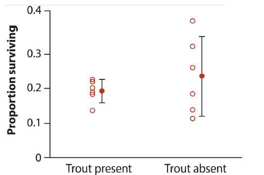
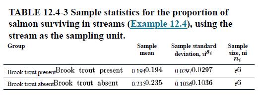
Figure 12.4-1 and the summary statistics in Table 12.4-3 show that streams without introduced trout have a sample standard deviation more than three times that of streams with trout. This is a case where the Welch’s approximate t-test is appropriate (see Section 12.3). Using Welch’s t-test and a computer, we find that t=0.93, df=5, and the P-value for the test is P=0.39. Hence, P>0.05 and we cannot reject the null hypothesis. In other words, the data do not support the claim that the brook trout lower the survivorship of chinook salmon. The lower and upper limits of the Welch’s 95% confidence interval for the difference between the means of these two groups are −0.07 and 0.15.

The appropriate analysis, in which salmon data within streams are reduced to a single measurement per stream, might seem like a waste of hardearned data. We started with survival data on 9211 salmon but used only six measurements per treatment. The contingency analysis rejected H₀, but the Welch’s two-sample test did not! Have we thrown away data and lost power as a result? There are two answers to this question. First, if the raw data are not randomly sampled, then it is not legitimate to analyze them as though they were a random sample. You can’t lose power that you never had. But the kinder, gentler answer is that the data are not wasted. By pooling together several related data points into a single summary measure, such as a proportion, you will have an increasingly reliable measure of the true value of that measure in a given sample unit, such as a stream. As a result, little or no information is “lost.”