The theory of scattering generalizes in a pretty obvious way to arbitrary localized potentials (Figure 2.21). To the left (Region I), V (x) = 0, so

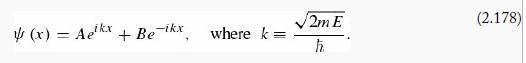
To the right (Region III), V (x) is again zero, so

In between (Region II), of course, I can’t tell you what is until you specify the potential, but because the Schrödinger equation is a linear, second-order differential equation, the general solution has got to be of the form

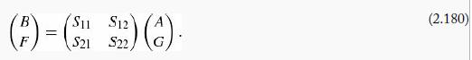
where f(x) and g (x) are two linearly independent particular solutions. There will be four boundary conditions (two joining Regions I and II, and two joining Regions II and III). Two of these can be used to eliminate C and D, and the other two can be “solved” for B and F in terms of A and G:

The four coefficients S_ij , which depend on k (and hence on E), constitute a 2 x 2 matrix S, called the scattering matrix (or S-matrix, for short). The S-matrix
tells you the outgoing amplitudes (B and F) in terms of the incoming amplitudes (A and G):

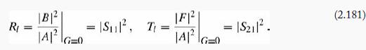
In the typical case of scattering from the left, G = 0, so the reflection and transmission coefficients are

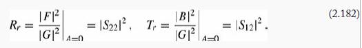
For scattering from the right, A = 0, and

(a) Construct the S-matrix for scattering from a delta-function well (Equation 2.117).
(b) Construct the S-matrix for the finite square well (Equation 2.148).

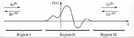
Figure 2.21: Scattering from an arbitrary localized potential (V (x) = 0 except in Region II); Problem 2.53.

Transcribed Image Text:

(x) = Ae¹kx + Be-ikx where k = 2m E ħ. (2.178)