Using the data provided in Example 2, fit the nonlinear model y = ae^–bx. How does this solution compare to the power model found in Example 2?

Data from example 2

Consider the following data on the average tread on a radial racing tire over time. The variable x will be the hours in heavy racing use, and the variable y will be the average tread thickness in centimeters (cm). The plot looks like the exponential decaying power function (Figure 13.11).

Figure 13.11

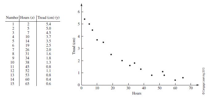
The graph of Figure 13.11 shows a decreasing trend that is concave upward. This suggests a model of the form y = ax^b. Using least squares, we want to minimize the sum of squared error:

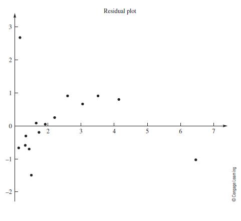
We take the partial derivatives with respect to the two parameters, a, and b. We cannot solve the resulting system of nonlinear equations to obtain a closed form solution. We can use the gradient search to estimate the values of the parameters and b. We use technology to obtain the numerical solution. We find, SSE = 6.62572; a = 8.879, and b = –0.46622. The generalized nonlinear model is 8.879x^–0.46622. We plot both the model and the data as well as the residuals in Figures 13.12 and 13.13 respectively. We accept the model as adequate as we find the model appears to fit well and we find no trend in the residuals. We might use the model to predict or interpolate.

Figure 13.12

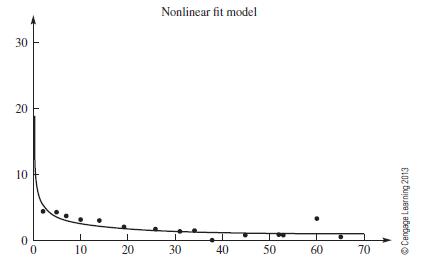
Figure 13.13

Transcribed Image Text:

Number Hours (x) |Tread (cm) (y) 123456rxgULSHS 7 8 9 10 2STOHAGENES 5 7 10 14 19 26 31 34 38 45 52 53 60 65 5.4 5.0 4.5 i Immicic 157 3.7 3.5 2.5 2.0 1.6 1.8 1.3 0.8 1.1 0.8 0.4 0.6 Tread (cm) 6 5 + 2 1 0 0 10 1 20 I 30 Hours 1 40 I 50 60 70 Cengage Leaming 2013