In this chapter, we discussed the relationship between height and wages in the United States. Does this pattern occur elsewhere? The data set heightwage_british_males.dta contains data on males in Britain from Persico, Postlewaite, and Silverman (2004). This data is from the British National Child Development Survey, which began as a study of children born in Britain during the week of March 3, 1985. Information was gathered when these subjects were 7, 11, 16, 23, and 33 years old. For this question, we use just the information about respondents at age 33. Table 3.5 shows the variables we use.

(a) Estimate a model where height at age 33 explains income at age 33. Explain \(\hat{\beta}_{1}\) and \(\hat{\beta}_{0}\).

(b) Create a scatterplot of height and income at age 33. Identify outliers.

Table 3.5:

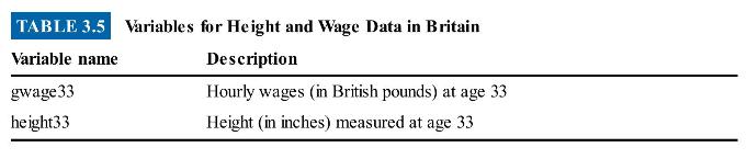
(c) Create a scatterplot of height and income at age 33, but exclude observations with wages per hour more than 400 British pounds and height less than 40 inches. Describe the difference from the earlier plot. Which plot seems the more reasonable basis for statistical analysis? Why?

(d) Reestimate the bivariate OLS model from part (a), but exclude four outliers with very high wages and outliers with height below 40 inches. Briefly compare results to earlier results.

(e) What happens when the sample size is smaller? To answer this question, reestimate the bivariate OLS model from above (that excludes outliers), but limit the analysis to the first 800 observations. Which changes more from the results with the full sample: the estimated coefficient on height or the estimated standard error of the coefficient on height? Explain.

Transcribed Image Text:

TABLE 3.5 Variables for Height and Wage Data in Britain Variable name gwage 33 height33 Description Hourly wages (in British pounds) at age 33 Height (in inches) measured at age 33