

The variables we will use are listed in Table 7.5. (a) Is the effect of age on
Question:
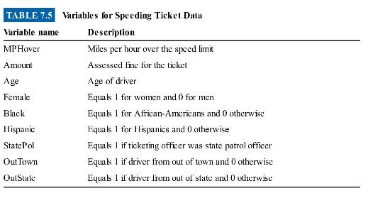
The variables we will use are listed in Table 7.5.
(a) Is the effect of age on fines non-linear? Assess this question by estimating a model with a quadratic age term, controlling for MPHover, Female, Black, and Hispanic. Interpret the coefficients on the age variables.
(b) Sketch the relationship between age and ticket amount from the foregoing quadratic model: calculate the fitted value for a white male with MPHover equals 0 (probably not many people going zero miles over the speed limit got a ticket, but this simplifies calculations a lot) for ages equal to \(20,25,30,35,40\), and 70 . (In Stata, the following displays the fitted value for a 20 -year-old, assuming all other independent variables equal zero: display _ b[_cons] + _b[Age]*20+_b[AgeSq]*20^2. In R, suppose that we name our OLS model in part
(a) "TicketOLS." Then the following displays the fitted value for a 20 -year-old, assuming all other independent variables equal zero: coef(TicketOLS) [1] + coef(TicketOLS) [2]*20 + coef(TicketOLS)[3]*(20^2).)
Use Equation 7.4 to calculate the marginal effect of age at ages 20,
\(\frac{\partial Y}{\partial X_1}=\beta_1+2 \beta_2 X_1 \tag{7.4}\)
(c) 35, and 70. Describe how these marginal effects relate to your sketch.
(d) Calculate the age that is associated with the lowest predicted fine based on the quadratic OLS model results given earlier.
(e) Do drivers from out of town and out of state get treated differently? Do state police and local police treat non-locals differently? Estimate a model that allows us to assess whether outof-towners and out-of-staters are treated differently and whether state police respond differently to out-of-towners and out-ofstaters. Interpret the coefficients on the relevant variables.
(f) Test whether the two state police interaction terms are jointly significant. Briefly explain the results.
Step by Step Answer:

This question has not been answered yet.
You can Ask your question!

Real Econometrics The Right Tools To Answer Important Questions
ISBN: 9780190857462
2nd Edition
Authors: Michael Bailey
