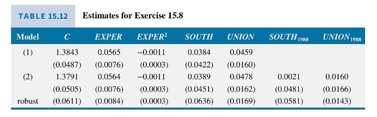
Using the NLS panel data on \(N=716\) young women, we are interested in the relationship between \(\ln (W A G E)\) and experience, its square, and indicator variables for living in the south and union membership. The equation of interest is (XR15.6) in Exercise 15.6. Some estimation results are in Table 15.12. The estimates are based on 2864 observations covering the years 1982, 1983, 1985, and 1987. Standard errors are in parentheses.

a. Explain why the strict form of exogeneity, FE2, is required for the fixed effects estimator to be consistent. You may wish to reread the start of Section 15.1.2 to help clarify the assumption.

b. The fixed effects estimates of the regression coefficients and conventional standard errors are reported as Model (1). Are the coefficients significantly different from zero at the 5\% level? What do the signs of the coefficients on experience and its square indicate about returns to experience?

c. In the fixed effects model, the assumption of strict exogeneity can be checked. Model (2) in Table 15.12 adds the variables SOUTH and UNION for year 1988 to the fixed effects equation and we report conventional standard and cluster-robust standard errors. As noted in equation (15.5a), the strict exogeneity assumption fails if the random error is correlated with the explanatory variables in any time period. We can check for such a correlation by including some, or all, of the explanatory variables for year \(t+1\) into the fixed effects model equation. If strict exogeneity holds these additional variables should not be significant. Based on the Model (2) result is there any evidence that the strict exogeneity assumption does not hold?

d. The joint \(F\)-test of SOUTH \(_{1988}\) and UNION \(_{1988}\) with conventional standard errors is 0.47 . What are the degrees of freedom for the \(F\)-test? What is the \(5 \%\) critical value? What do we conclude about strict exogeneity based on the joint test?

e. The joint \(F\)-test of \(S^{2} O T H_{1988}\) and \(U_{19} O_{1988}\) with robust-cluster standard errors is 0.63 . When using a cluster-corrected covariance matrix the \(F\)-statistic used by some software has \(M-1\) denominator degrees of freedom, where \(M\) is the number of clusters. In this case, what is the \(5 \%\) critical value? What do we conclude about strict exogeneity based on the robust joint test?

Data From Exercise 15.6:-

Using the NLS panel data on \(N=716\) young women, we consider only years 1987 and 1988 . We are interested in the relationship between \(\ln (W A G E)\) and experience, its square, and indicator variables for living in the south and union membership. Some estimation results are in Table 15.10.

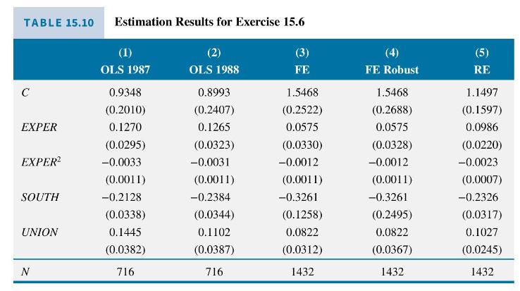
a. The OLS estimates of the \(\ln (W A G E)\) model for each of the years 1987 and 1988 are reported in columns (1) and (2). How do the results compare? For these individual year estimations, what are you assuming about the regression parameter values across individuals (heterogeneity)?

b. The \(\ln (W A G E)\) equation specified as a panel data regression model is

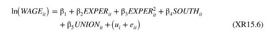
Explain any differences in assumptions between this model and the models in part (a).

c. Column (3) contains the estimated fixed effects model specified in part (b). Compare these estimates with the OLS estimates. Which coefficients, apart from the intercepts, show the most difference?

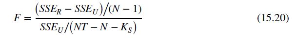
d. The \(F\)-statistic for the null hypothesis that there are no individual differences, equation (15.20), is 11.68. What are the degrees of freedom of the \(F\)-distribution if the null hypothesis (15.19) is true? What is the \(1 \%\) level of significance critical value for the test? What do you conclude about the null hypothesis.

e. Column (4) contains the fixed effects estimates with cluster-robust standard errors. In the context of this sample, explain the different assumptions you are making when you estimate with and without cluster-robust standard errors. Compare the standard errors with those in column (3). Which ones are substantially different? Are the robust ones larger or smaller?

f. Column (5) contains the random effects estimates. Which coefficients, apart from the intercepts, show the most difference from the fixed effects estimates? Use the Hausman test statistic (15.36) to test whether there are significant differences between the random effects estimates and the fixed effects estimates in column (3) (Why that one?). Based on the test results, is random effects estimation in this model appropriate?

Data From Equation 15.20:-

Transcribed Image Text:

TABLE 15.12 Estimates for Exercise 15.8 Model C EXPER EXPER SOUTH UNION SOUTH 1988 UNION 1988 (1) 1.3843 0.0565 -0.0011 0.0384 0.0459 (0.0487) (0.0076) (0.0003) (0.0422) (0.0160) (2) 1.3791 0.0564 -0.0011 0.0389 0.0478 0.0021 0.0160 (0.0505) (0.0076) (0.0003) (0.0451) (0.0162) (0.0481) (0.0166) robust (0.0611) (0.0084) (0.0003) (0.0636) (0.0169) (0.0581) (0.0143)