In this problem, you will use your knowledge of solving systems of ordinary differential equations and phase planes to look at the classic predator–prey problem in biology. The model itself is very simple and covered in numerous textbooks on biology, population dynamics, and nonlinear analysis. Let x be the population of prey and y be the population of predators. The rate of change of these populations is modeled by the coupled set of ordinary differential equations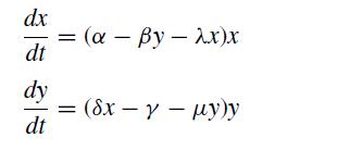

The parameters α, β, λ, δ, γ , and μ are positive. Naturally, the predator population y and prey population x cannot be negative.

If we think about the left-hand side as the growth of each population, then we can interpret the different terms as follows:

• The terms αx − λx² ensure that the prey population grows if it is small but decays when it gets large

• The term −βxy decreases the prey population as both the predator and the prey become abundant

• The terms δx − γ increases the predator population if there is more prey to eat and decreases it when there is not enough food

• The term −μy² decreases the predator population as it gets large.

The problem can be put in a “dimensionless” form through the transformations τ = αt, u = δx/α, and v = βy/α. This is not really a dimensional analysis of the type you see in transport phenomena, for example, but it does reduce the number of parameters to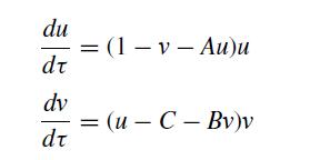

(a) Determine how the parameters A, B, and C are related to the original parameter set α, β, λ, δ, γ , and μ.

(b) One possible steady state for this system is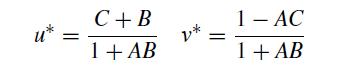

Confirm that this is a steady state solution. Do we need to put any restrictions on these parameter values to ensure that the stable points are non-negative?

(c) For the following values of A, B, and C, calculate the corresponding steady state values of u^∗ and v^∗.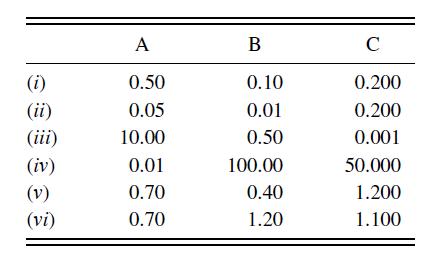

You can either make the calculation by hand or use a MATLAB program to make the calculations using the result from part (b). Use MATLAB to create a plot (v vs. u) using a circle to mark each steady state. Are there bounds on the possible steady state values of u^∗ and v^∗?

(d) Determine the entries of the Jacobian as a function of A, B, C, u, and v. Using the values of A, B, and C from the table above, perform a linear stability analysis from this Jacobian and determine the eigenvalues for each case near the steady state. What do the eigenvalues for each of these cases tell you (qualitatively) about the stability of the steady states?

(e) Write a MATLAB program that integrates the governing equations using a fourth order Runge–Kutta method. Produce a phase plot for each of the above sets of A, B, and C with initial conditions u(0) = 2 and v(0) = 2. Use 0.01 as the dimensionless time step and integrate until you reach a distance of r = 10⁻⁴ from the steady state solution. If the solution becomes unstable, repeat the calculation by sequentially halving the time step until the time integration is stable. Include in your code a way to count the number of oscillations for those solutions which are oscillatory. Note the time step required to have a stable integration for each of the phase planes.

Transcribed Image Text:

dx dt dy dt = (x -By-dx)x (8x - y - Lyy