In this problem, you will use your knowledge of the phase plane and stability to analyze a simple model of glycolysis. The glycolysis pathway that first convert glucose into fructose-6-phosphate (F6P), and later lead to two molecules of pyruvate, which then enters the TCA cycle. In the course of the reaction, there are reactions which convert ATP to ADP, as well as the reverse reactions.

A simplified model of glycolysis considers only the concentrations of ADP, which we will call x, and the concentration of F6P, which we will call y. The model equations are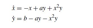

where a and b are positive coefficients. The goal of this problem is to analyze the dynamics of this simplified model of glycolysis.

This problem consists of two parts. The first one is primarily analytical with some programming tasks to assist in your analysis. The second one is primarily computational. While both parts refer to the same problem, you can probably do most of the second one without doing the first one. So if you get stuck early on, don’t neglect the second part.

Part I

In the first part of the problem, we will analyze the stability of the steady states of this reaction system. The final result will be a detailed output file, along with two plots if you do the bonus activity. Your final program will be a function called stability, which calls a subfunction called eigenval.

(a) Determine the steady state of this system, the Jacobian at steady state, and the eigenvalues at steady state. Include your calculation in the written submission.

(b) Determine the boundary between the stable and unstable steady states in the problem. Include your calculation in the written submission. Hint: If you are having trouble with this calculation, you should do the numerical calculations below. If you can do them successfully, it may help you to see the answer to this part of the problem.

(c) Write a MATLAB function called eigenval(a,b) that takes as its inputs the parameters a and b. The function should return a vector containing the following outputs (in this order).

(1) The real part of the larger eigenvalue.

(2) The imaginary part of the larger eigenvalue.

(3) The real part of the smaller eigenvalue.

(4) The imaginary part of the smaller eigenvalue.

(5) A number indicating the type of steady state: 1 = stable node, 2 = unstable node, 3 = saddle point, 4 = stable spiral, 5 = unstable spiral, 6 = center.

Since you will never actually get a center in a numerical calculation, if the real part of the eigenvalues is less than 10−6, you can assume that the steady state is a center. In this calculation, you are not allowed to use the imaginary number capabilities of MATLAB. You should construct your function with conditional if-else type statements to determine the real and imaginary parts, as well as the type of eigenvalue.

(d) Write a MATLAB function called stability for analyzing the steady states. This function must call your eigenval function for the relevant calculations. You are to consider all combinations of the values a = 0.005, 0.010,. . ., 0.14 and b = 0.05, 0.1, . . ., 1.2. For each (a, b) pair, this function should compute the steady state (x_ss,y_ss), the real and imaginary parts of each eigenvalue, and the type of steady state using the numbering system defined above. Compile all of these data into a matrix whose columns correspond to the following:

(1) a.

(2) b.

(3) The steady state value xss.

(4) The steady state value yss.

(5) The real part of the larger eigenvalue.

(6) The imaginary part of the larger eigenvalue.

(7) The real part of the smaller eigenvalue.

(8) The imaginary part of the smaller eigenvalue.

(9) A number indicating the type of steady state: 1 = stable node, 2 = unstable node, 3 = saddle point, 4 = stable spiral, 5 = unstable spiral, 6 = center.

The matrix should be saved to a file using dlmwrite.

Bonus: Have your program create the following plots.

(1) A plot of the type of steady state in the x, y plane. Use blue color for stable states, red color for unstable states, circles for nodes, x for spirals, a green triangle for a saddle point, and a black pentagram for a center. Label the axes, provide a title, and save the plot as a jpg. Hint: Do not worry if you have trouble seeing all of the steady states in your plot. If you look back at your answers for the values of the steady state as a function of a and b, it may help you understand this plot.

(2) A plot of the type of steady state in the a, b plane. Use blue color for stable states, red color for unstable states, circles for nodes, x for spirals, a green triangle for a saddle point, and a black pentagram for a center. You should also plot the boundary of the stability envelope in the second figure. Label the axes, provide a title, and save the plot as a jpg.

If you have many different conditions, it is easier to use a switch statement than a bunch of if-else statements. In order to make plots using different types of symbols, you should use the hold on and hold off commands. You can get a very deep understanding of the stability of this problem from these plots, which is why you should try to make them. However, the plotting is included as extra credit because it involves a reasonably good understanding of MATLAB plotting commands.

Part II

In the second part of the problem, you will construct three phase diagrams for particular conditions of a, b, and initial conditions. The various conditions are in Table 5.1. You will need to construct phase planes for these conditions using RK4 and explain the results. Your final program will a function called makeplots that calls the subfunctions RK4, RK, and feval.

(a) Write a MATLAB function called feval(z,a,b) that takes in a vector of positions z = [x, y] and the parameters a, b and returns the values of ˙x and ˙y.

(b) Write a MATLAB function called RK(z,h,a,b) that takes in a vector of the current values z, the time step h, and the parameters a and b and returns the new values of z. Your function must call feval(z,a,b) to compute the various k values.

(c) Write a MATLAB function called RK4(a,b,z) that takes in a vector initial positions z = [x0, y0] and the parameters a and b and performs RK4 for 104 time steps with a step size h = 0.01. The function should plot the starting point as a blue circle and the trajectory as a blue line. Your function must call RK(z,h,a,b) for the integration.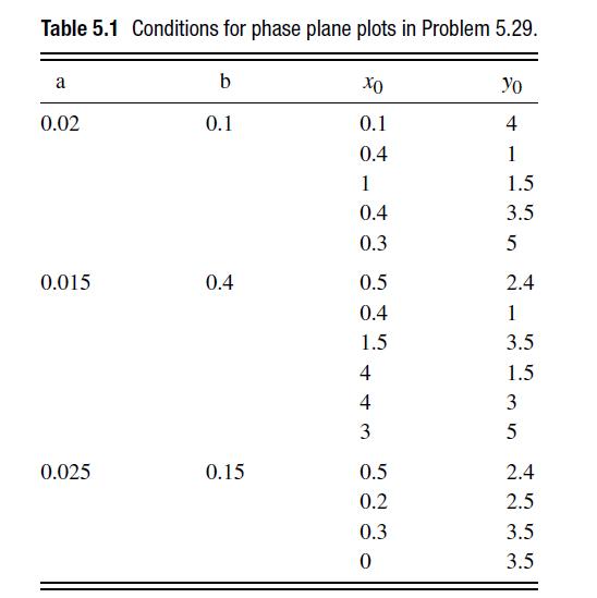

(d) Write a MATLAB function called makeplots that will create the phase planes. For each case, you should plot the steady state as a red x and then have each trajectory plotted from the RK4(a,b,z) function. These extra points make it easier to see the direction of the trajectory. Label the axes, provide a title and save each plot as a jpg file. Hint: In order to make plots using different types of symbols, you should use the hold on and hold off commands.

(e) Explain the result of each phase plane.

Transcribed Image Text:

x = -x +ay+x²y y=b-ay-x²y