This problem considers different aspects of the solution of the unsteady heat equation.

(a) Use separation of variables to solve the PDE

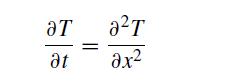
with no flux boundary conditions at x = 0 and x = 1 and an initial condition T = 1 − x.

(b) Write a MATLAB program that makes a plot of T(x, t) versus x for a given value of t and a number n of non-zero terms in the Fourier series. You should use 200 grid points for x. We want to explore the error in the solution as a function of n. Let us define the error as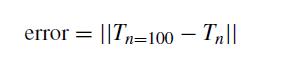

where T_n is the temperature field with n terms in the Fourier series. Naturally, the error will go to zero when you have 100 terms, since this definition assumes that n = 100 is sufficient.

(c) Have your program automatically generate a log–log plot of the error versus the number of terms in the series for n = 1 to n = 99 for two different values of the time, t = 0.000 05 and t = 0.001. Explain why these two curves are different.

(d) Now investigate the cost of solving the PDE in part (a) using centered finite differences. First write a code that uses RK4 to perform the integration with ten grid points in x. Your program should automatically plot the numerical solution at the times t = 0, 0.01, 0.05, 0.1, and 0.5. It should also make a plot of the exact solution at these times using n = 100 terms in the Fourier series. The purpose of this part of the problem is for you to confirm that your code works correctly – even for a very coarse discretization the numerical solution is very close to the exact solution.

Transcribed Image Text:

aT а т at ах2 =