This problem involves the solution of the diffusion equation

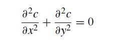
with no flux boundary conditions at x = 0 and x = 1 and a concentration c = 1 at y = 1. The end goal is to determine the concentration profile when the boundary condition at y = 0 is zero for x ∈ [0, 0.25] and x ∈ [0.5, 0.75] and no-flux otherwise. The first two parts are designed to help you debug your code, and the third part is the goal of the problem.

(a) Write a MATLAB program that uses finite differences to solve this problem where the boundary condition at y = 0 is c = 0. Your program should automatically generate a plot of the concentration as a function of position. A convenient plotting tool is mesh, which requires that you have your concentration in the form of a matrix. You can also provide matrices with the corresponding x and y data to make a nicely formatted plot. What is the exact solution to the problem?

(b) Now modify your program to use no-flux at y = 0. In addition to plotting the solution, display the values of the concentration to the screen. (This will help with your interpretation of the result.) What are the new boundary equations and the exact result for this problem?

(c) Now modify your program to use c = 0 at y = 0 for x ∈ [0, 0.25] and x ∈ [0.5, 0.75] and no-flux otherwise. You program should produce two plots. The first plot is the same as the previous problems, with the concentration as a function of twodimensional position. The second plot is the concentration at the lower boundary, c(x, 0), as a function of x. What was your method for implementing the lower boundary condition?

Transcribed Image Text:

a²c a2c 2с ах2 ду2 + = 0