

1 2 The Week worksheet contains data for the week of April 5. In cell D7, insert...
Question:
1 |
|
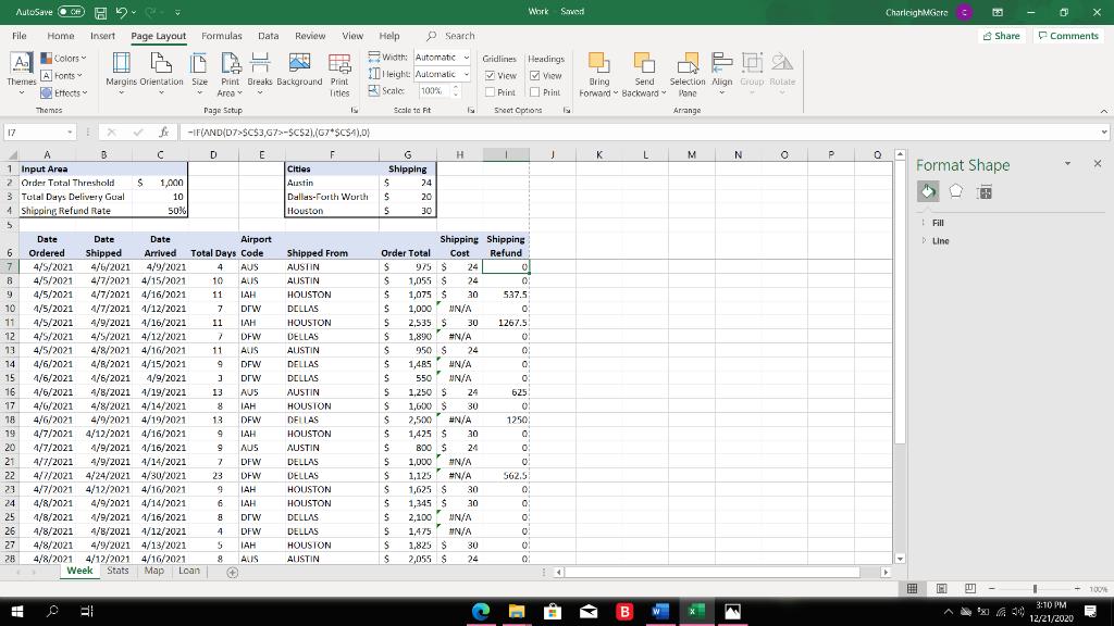
2 | The Week worksheet contains data for the week of April 5. |
3 | Next, you want to display the city names that correspond with the city airport codes. |
4 | Now you want to display the standard shipping costs by city. |
5 | Finally, you want to calculate a partial shipping refund if two conditions are met. |
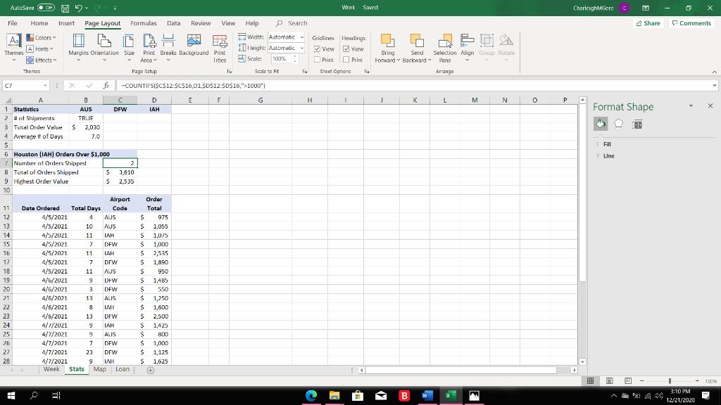
6 | The Stats worksheet contains similar data. Now you want to enter summary statistics. |
7 | In cell B3, insert the SUMIF function to calculate the total orders for Austin (cell B1). Use appropriate mixed references to the range argument to keep the column letters the same. Copy the function to the range C3:D3. |
8 | In cell B4, insert the AVERAGEIF function to calculate the average number of days for shipments from Austin (cell B1). Use appropriate mixed references to the range argument to keep the column letters the same. Copy the function to the range C4:D4. |
9 | Now you want to focus on shipments from Houston where the order was greater than $1,000. |
10 | In cell C8, insert the SUMIFS function to calculate the total orders where the Airport Code is IAH (Cell D1) and the Order Total is greater than $1,000. |
11 | In cell C9, insert the MAXIFS function to return the highest order total where the Airport Code is IAH (Cell D1) and the Order Total is greater than $1,000. |
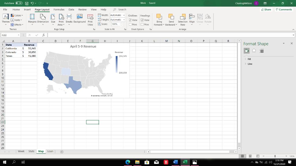
12 | On the Map worksheet, insert a map for the states and revenues. Cut and paste the map in cell C1. |
13 | Format the data series to show only regions with data and show all map labels. |
14 | Change the map title to April 5-9 Gross Revenue. |
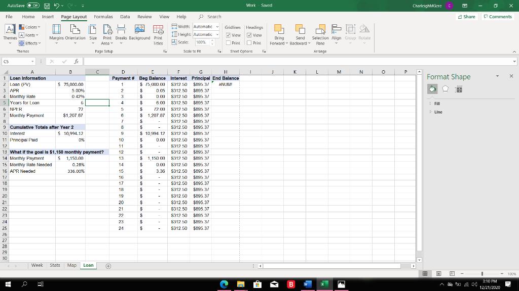
15 | Use the Loan worksheet to complete the loan amortization table. |
16 | In cell G2, insert the PPMT function to calculate the principal paid for the first payment. Copy the function to the range G3:G25. |
17 | In cell H2, insert a formula to calculate the ending principal balance. Copy the formula to the range H3:H25. |
18 | Now you want to determine how much interest was paid during the first two years. |
19 | In cell B11, insert the CUMPRINC function to calculate the cumulative principal paid at the end of the first two years. Make sure the result is positive. |
20 | You want to perform a what-if analysis to determine the rate if the monthly payment is $1,150 instead of $1,207.87. |
21 | Finally, you want to convert the monthly rate to an APR. |
22 | Insert a footer on all sheets with your name on the left side, the sheet name code in the center, and the file name code on the right side. |
23 | Save and close Exp19_Excel_Ch07_CapAssessment_Shipping.xlsx. Exit Excel. Submit the file as directed. |
Expert Answer:


Elementary Statistics
ISBN: 978-0538733502
11th edition
Authors: Robert R. Johnson, Patricia J. Kuby
