

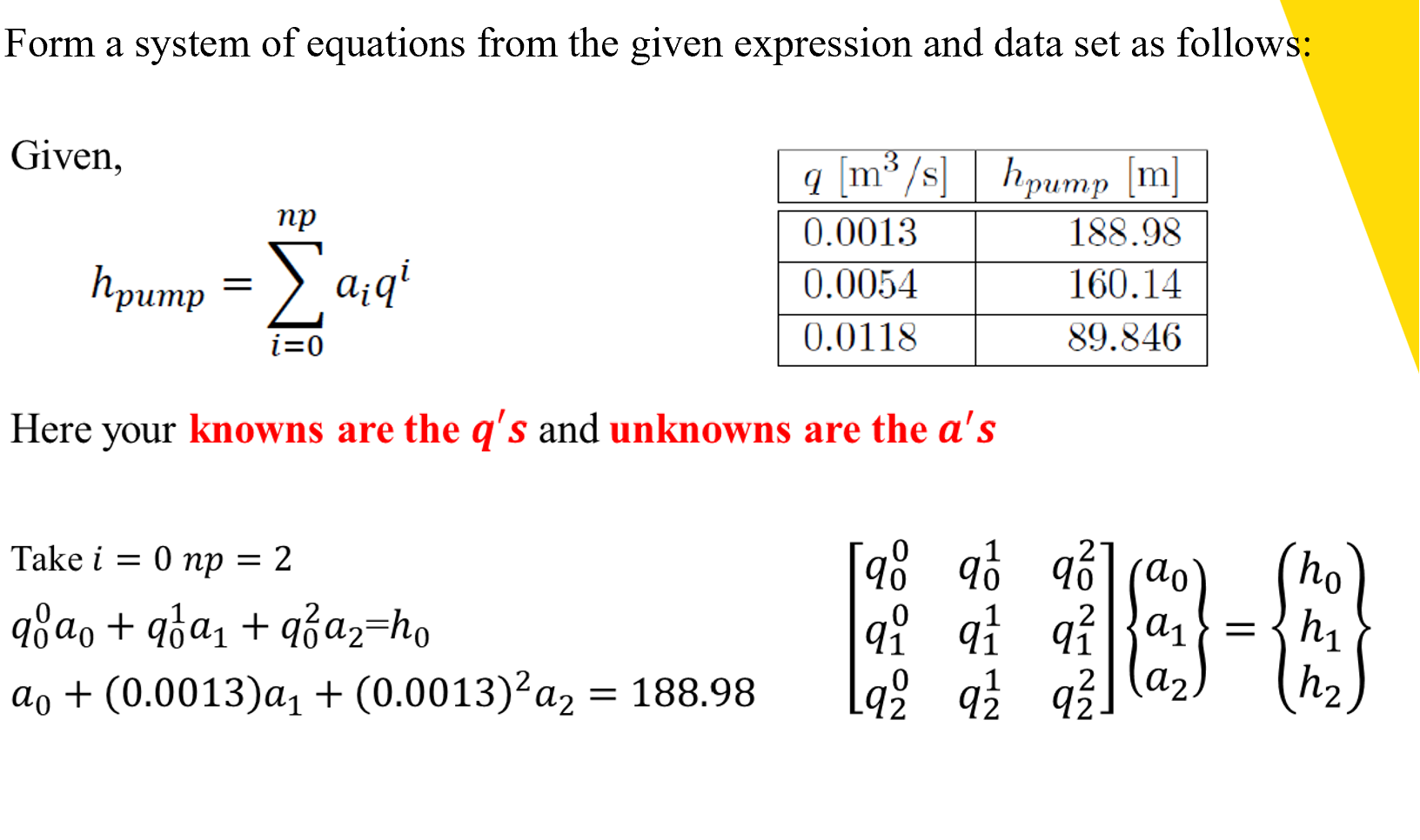
Form a system of equations from the given expression and data set as follows: Given, np...
Fantastic news! We've Found the answer you've been seeking!
Question:
Transcribed Image Text:
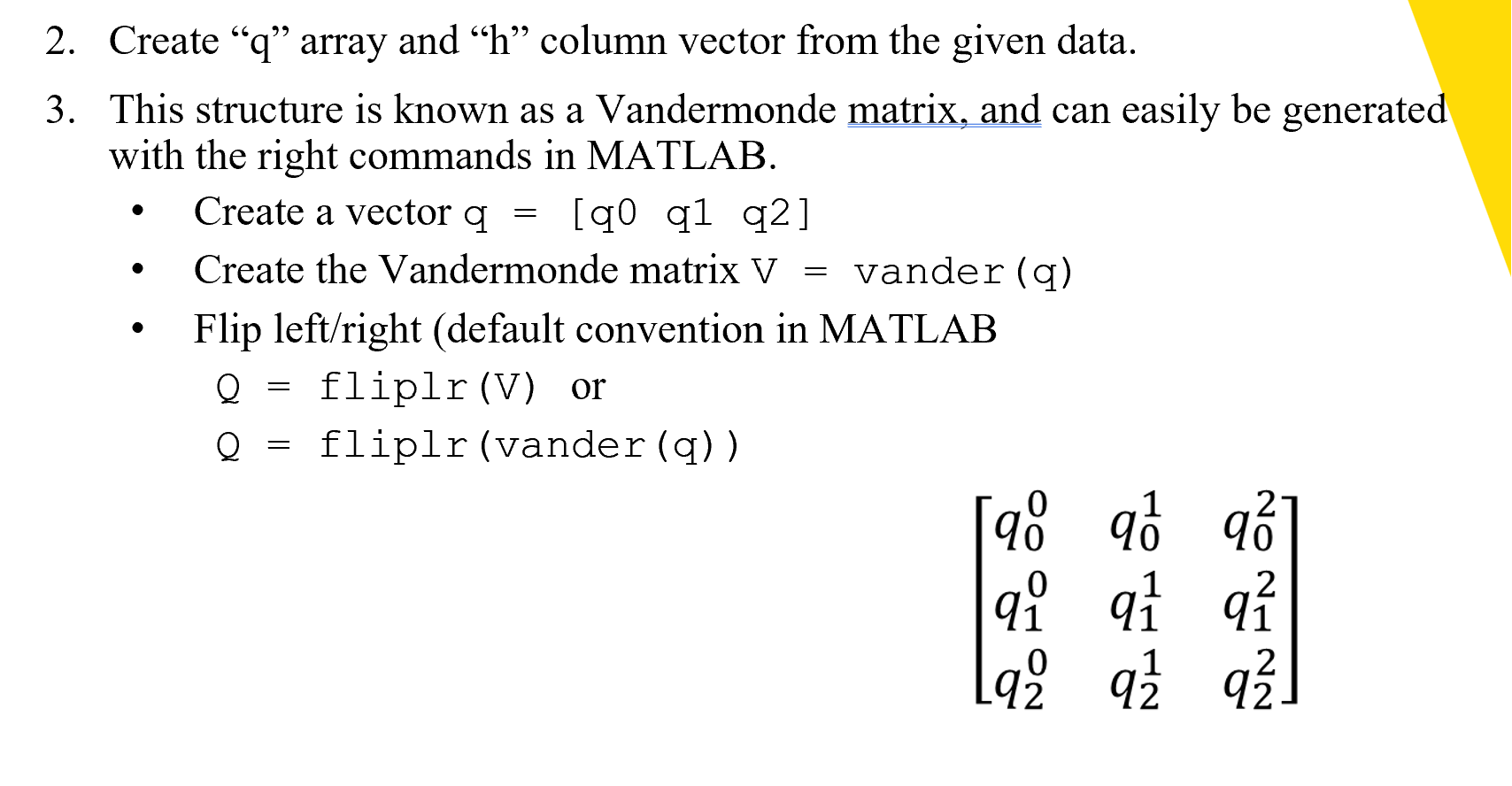
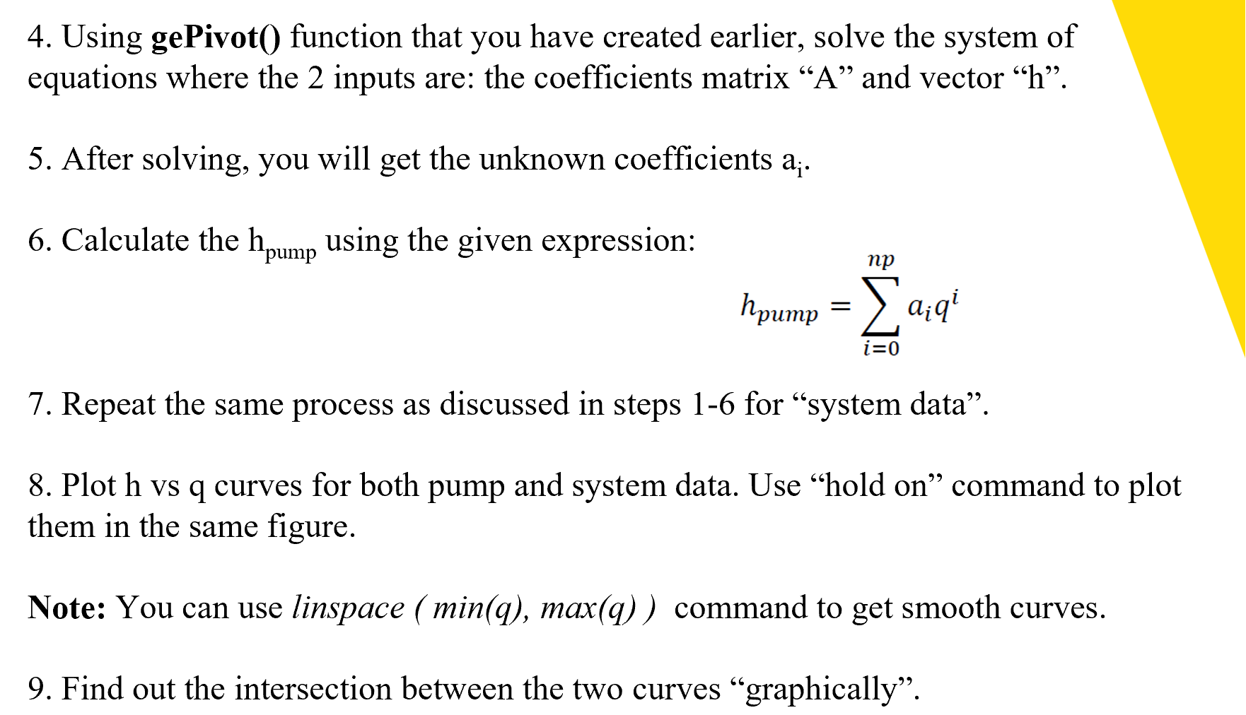
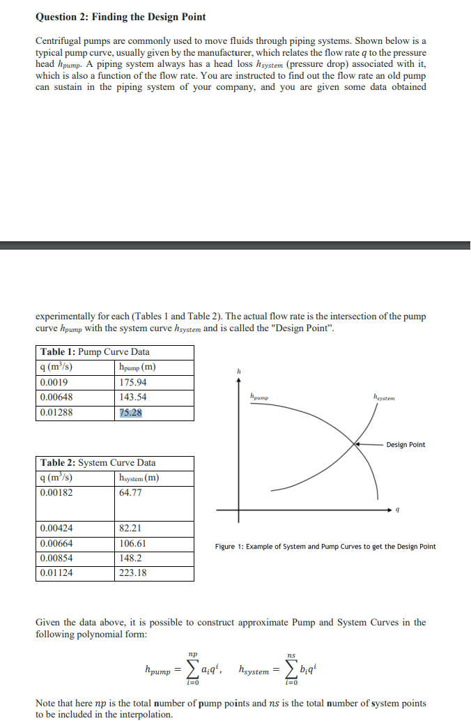
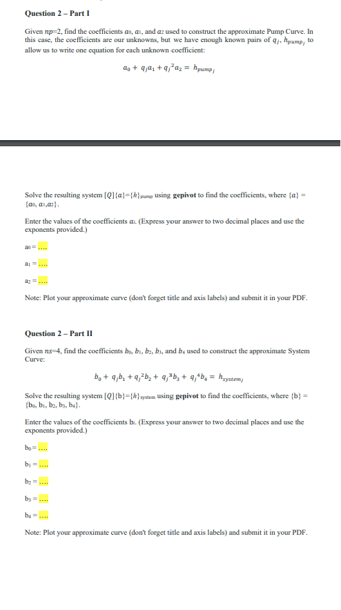
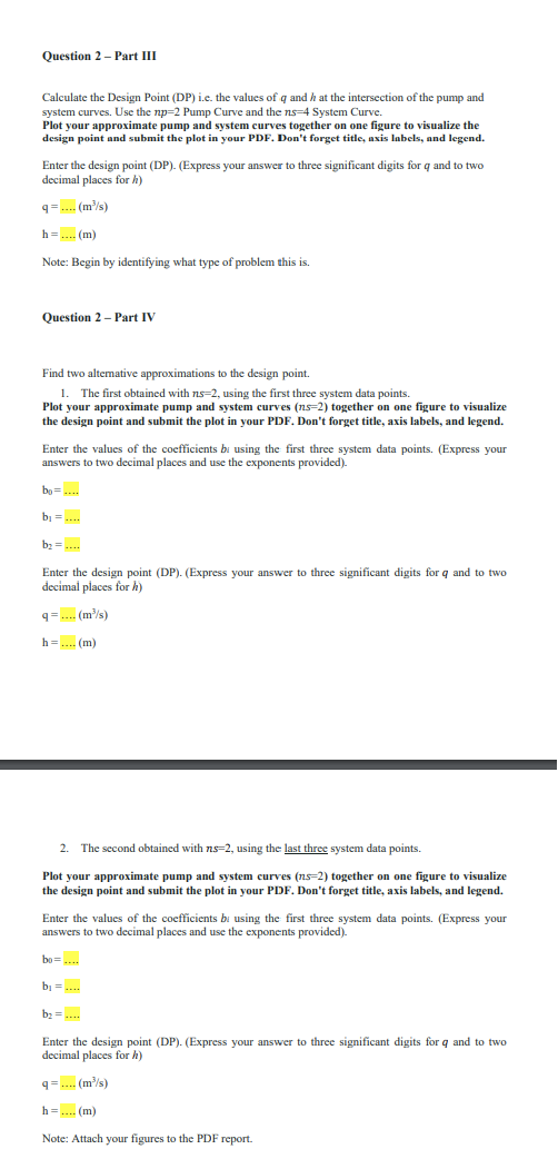
Form a system of equations from the given expression and data set as follows: Given, np hpump = [aq i=0 q [m/s] hpump [m] 188.98 160.14 89.846 Take i = 0 np = 2 qao + qa + qa=ho ao + (0.0013) a + (0.0013)a = 188.98 0.0013 0.0054 0.0118 Here your knowns are the q's and unknowns are the a's 0 9 91 0 91 9 q1 92 9/2 9] (ao q 9a}= (a) 2 q 9. 2 ho h h 2. Create "q" array and h column vector from the given data. 3. This structure is known as a Vandermonde matrix, and can easily be generated with the right commands in MATLAB. Create a vector q [q0 q1 q2] Create the Vandermonde matrix V = vander (q) Flip left/right (default convention in MATLAB Q fliplr (V) or Q fliplr (vander (q)) = = = 0 [98 0 qi 2 996 2 q1 q 0 2 92 9 9 4. Using gePivot() function that you have created earlier, solve the system of equations where the 2 inputs are: the coefficients matrix "A" and vector h. 5. After solving, you will get the unknown coefficients a. 6. Calculate the hpump using the given expression: np hpump = aq i=0 7. Repeat the same process as discussed in steps 1-6 for "system data. 8. Plot h vs q curves for both pump and system data. Use "hold on" command to plot them in the same figure. Note: You can use linspace (min(q), max(q)) command to get smooth curves. 9. Find out the intersection between the two curves "graphically". Question 2: Finding the Design Point Centrifugal pumps are commonly used to move fluids through piping systems. Shown below is a typical pump curve, usually given by the manufacturer, which relates the flow rate q to the pressure head hpump. A piping system always has a head loss hsystem (pressure drop) associated with it, which is also a function of the flow rate. You are instructed to find out the flow rate an old pump can sustain in the piping system of your company, and you are given some data obtained experimentally for each (Tables 1 and Table 2). The actual flow rate is the intersection of the pump curve hpump with the system curve hsystem and is called the "Design Point". Table 1: Pump Curve Data q (m/s) 0.0019 0.00648 0.01288 hpump (m) 175.94 143.54 75.28 Table 2: System Curve Data q (m/s) hsystem (m) 0.00182 64.77 0.00424 0.00664 0.00854 0.01124 82.21 106.61 148.2 223.18 hpump np hpump = [9;9, hsystem = i=0 heystem Figure 1: Example of System and Pump Curves to get the Design Point i=0 Design Point Given the data above, it is possible to construct approximate Pump and System Curves in the following polynomial form: biq 9 Note that here np is the total number of pump points and ns is the total number of system points to be included in the interpolation. Question 2 - Part I Given np-2, find the coefficients ao, ai, and az used to construct the approximate Pump Curve. In this case, the coefficients are our unknowns, but we have enough known pairs of qj, hpump, to allow us to write one equation for each unknown coefficient: ao+qja + aa=hpump, Solve the resulting system [Q]{a}={hpump using gepivot to find the coefficients, where {a} = {ai, ai,az). Enter the values of the coefficients al. (Express your answer to two decimal places and use the exponents provided.) al Note: Plot your approximate curve (don't forget title and axis labels) and submit it in your PDF. Question 2 - Part II Given ns-4, find the coefficients bo, bi, b2, b3, and b4 used to construct the approximate System Curve: bo+qb+q,b + q,b+ qjb = hsystem/ Solve the resulting system [Q] {b}={k} system using gepivot to find the coefficients, where {b} = {bo, bi, bz, bs, b4). Enter the values of the coefficients b. (Express your answer to two decimal places and use the exponents provided.) bo= b = b = b3 = b4 =.... Note: Plot your approximate curve (don't forget title and axis labels) and submit it in your PDF. Question 2 - Part III Calculate the Design Point (DP) i.e. the values of q and h at the intersection of the pump and system curves. Use the np-2 Pump Curve and the ns-4 System Curve. Plot your approximate pump and system curves together on one figure to visualize the design point and submit the plot in your PDF. Don't forget title, axis labels, and legend. Enter the design point (DP). (Express your answer to three significant digits for q and to two decimal places for h) q=.... (m/s) h =.... (m) Note: Begin by identifying what type of problem this is. Question 2 - Part IV Find two alternative approximations to the design point. 1. The first obtained with ns-2, using the first three system data points. Plot your approximate pump and system curves (ns-2) together on one figure to visualize the design point and submit the plot in your PDF. Don't forget title, axis labels, and legend. Enter the values of the coefficients be using the first three system data points. (Express your answers to two decimal places and use the exponents provided). bo= .... b =.... b =.... Enter the design point (DP). (Express your answer to three significant digits for q and to two decimal places for h) q=.... (m/s) h.... (m) 2. The second obtained with ns-2, using the last three system data points. Plot your approximate pump and system curves (ns-2) together on one figure to visualize the design point and submit the plot in your PDF. Don't forget title, axis labels, and legend. Enter the values of the coefficients bi using the first three system data points. (Express your answers to two decimal places and use the exponents provided). bo= .... b =.... b =.... Enter the design point (DP). (Express your answer to three significant digits for q and to two decimal places for h) = .... (m/s) h=.... (m) Note: Attach your figures to the PDF report. Form a system of equations from the given expression and data set as follows: Given, np hpump = [aq i=0 q [m/s] hpump [m] 188.98 160.14 89.846 Take i = 0 np = 2 qao + qa + qa=ho ao + (0.0013) a + (0.0013)a = 188.98 0.0013 0.0054 0.0118 Here your knowns are the q's and unknowns are the a's 0 9 91 0 91 9 q1 92 9/2 9] (ao q 9a}= (a) 2 q 9. 2 ho h h 2. Create "q" array and h column vector from the given data. 3. This structure is known as a Vandermonde matrix, and can easily be generated with the right commands in MATLAB. Create a vector q [q0 q1 q2] Create the Vandermonde matrix V = vander (q) Flip left/right (default convention in MATLAB Q fliplr (V) or Q fliplr (vander (q)) = = = 0 [98 0 qi 2 996 2 q1 q 0 2 92 9 9 4. Using gePivot() function that you have created earlier, solve the system of equations where the 2 inputs are: the coefficients matrix "A" and vector h. 5. After solving, you will get the unknown coefficients a. 6. Calculate the hpump using the given expression: np hpump = aq i=0 7. Repeat the same process as discussed in steps 1-6 for "system data. 8. Plot h vs q curves for both pump and system data. Use "hold on" command to plot them in the same figure. Note: You can use linspace (min(q), max(q)) command to get smooth curves. 9. Find out the intersection between the two curves "graphically". Question 2: Finding the Design Point Centrifugal pumps are commonly used to move fluids through piping systems. Shown below is a typical pump curve, usually given by the manufacturer, which relates the flow rate q to the pressure head hpump. A piping system always has a head loss hsystem (pressure drop) associated with it, which is also a function of the flow rate. You are instructed to find out the flow rate an old pump can sustain in the piping system of your company, and you are given some data obtained experimentally for each (Tables 1 and Table 2). The actual flow rate is the intersection of the pump curve hpump with the system curve hsystem and is called the "Design Point". Table 1: Pump Curve Data q (m/s) 0.0019 0.00648 0.01288 hpump (m) 175.94 143.54 75.28 Table 2: System Curve Data q (m/s) hsystem (m) 0.00182 64.77 0.00424 0.00664 0.00854 0.01124 82.21 106.61 148.2 223.18 hpump np hpump = [9;9, hsystem = i=0 heystem Figure 1: Example of System and Pump Curves to get the Design Point i=0 Design Point Given the data above, it is possible to construct approximate Pump and System Curves in the following polynomial form: biq 9 Note that here np is the total number of pump points and ns is the total number of system points to be included in the interpolation. Question 2 - Part I Given np-2, find the coefficients ao, ai, and az used to construct the approximate Pump Curve. In this case, the coefficients are our unknowns, but we have enough known pairs of qj, hpump, to allow us to write one equation for each unknown coefficient: ao+qja + aa=hpump, Solve the resulting system [Q]{a}={hpump using gepivot to find the coefficients, where {a} = {ai, ai,az). Enter the values of the coefficients al. (Express your answer to two decimal places and use the exponents provided.) al Note: Plot your approximate curve (don't forget title and axis labels) and submit it in your PDF. Question 2 - Part II Given ns-4, find the coefficients bo, bi, b2, b3, and b4 used to construct the approximate System Curve: bo+qb+q,b + q,b+ qjb = hsystem/ Solve the resulting system [Q] {b}={k} system using gepivot to find the coefficients, where {b} = {bo, bi, bz, bs, b4). Enter the values of the coefficients b. (Express your answer to two decimal places and use the exponents provided.) bo= b = b = b3 = b4 =.... Note: Plot your approximate curve (don't forget title and axis labels) and submit it in your PDF. Question 2 - Part III Calculate the Design Point (DP) i.e. the values of q and h at the intersection of the pump and system curves. Use the np-2 Pump Curve and the ns-4 System Curve. Plot your approximate pump and system curves together on one figure to visualize the design point and submit the plot in your PDF. Don't forget title, axis labels, and legend. Enter the design point (DP). (Express your answer to three significant digits for q and to two decimal places for h) q=.... (m/s) h =.... (m) Note: Begin by identifying what type of problem this is. Question 2 - Part IV Find two alternative approximations to the design point. 1. The first obtained with ns-2, using the first three system data points. Plot your approximate pump and system curves (ns-2) together on one figure to visualize the design point and submit the plot in your PDF. Don't forget title, axis labels, and legend. Enter the values of the coefficients be using the first three system data points. (Express your answers to two decimal places and use the exponents provided). bo= .... b =.... b =.... Enter the design point (DP). (Express your answer to three significant digits for q and to two decimal places for h) q=.... (m/s) h.... (m) 2. The second obtained with ns-2, using the last three system data points. Plot your approximate pump and system curves (ns-2) together on one figure to visualize the design point and submit the plot in your PDF. Don't forget title, axis labels, and legend. Enter the values of the coefficients bi using the first three system data points. (Express your answers to two decimal places and use the exponents provided). bo= .... b =.... b =.... Enter the design point (DP). (Express your answer to three significant digits for q and to two decimal places for h) = .... (m/s) h=.... (m) Note: Attach your figures to the PDF report.
Expert Answer:

Related Book For 

Discovering Advanced Algebra An Investigative Approach
ISBN: 978-1559539845
1st edition
Authors: Jerald Murdock, Ellen Kamischke, Eric Kamischke
Posted Date:
Students also viewed these mechanical engineering questions
-
CANMNMM January of this year. (a) Each item will be held in a record. Describe all the data structures that must refer to these records to implement the required functionality. Describe all the...
-
The following additional information is available for the Dr. Ivan and Irene Incisor family from Chapters 1-5. Ivan's grandfather died and left a portfolio of municipal bonds. In 2012, they pay Ivan...
-
Examine the articles reproduced below and consider how the five C's discussed in the course have application in the present coronavirus pandemic. "To the extent that an environment characterized by...
-
State the factor and the number of levels for the factor in each of the following tests. (a) A marine biologist measures the effectiveness of mating displays among tortoises in one of six...
-
Use the frequency histogram to (a) Determine the number of classes. (b) Estimate the greatest and least frequencies. (c) Determine the class width. (d) Describe any patterns with the data. Roller...
-
A lossless motor drives the fan shown in Fig. P12.40 at \(40 \mathrm{~Hz}\). The power input to the motor is \(40 \mathrm{amps}\) at 440 volts. For the geometry shown, what is the discharge flow rate...
-
Portfolio Expected Return you have $10,000 to invest in a stock portfolio. Your choices are Stock X with an expected return of 15 percent and Stock Y with an expected return of 10 percent. If your...
-
What are the environmental and safety considerations associated with the use of toxic or hazardous solvents in extraction processes, and how have green extraction techniques been developed to address...
-
1) Define what a "pantheon" is in 2-3 sentences in YOUR own words. 2) What was your favorite pantheon studied in this week's reading and why? (2-3 sentences) The Greek & Roman Pantheons, the...
-
1. Debug the following code by compiling it for debugging and executing it within a debugger. At which line of code does the program crash? Why does it crash there? #include #include main(int argc,...
-
Marketing mix analysis mini-study case for BMW company 1- Brand Management: Describe the company's 3 Cs of its brand communication, contribution, and competitive advantage; the concept of brand...
-
Consider the following ambiguous grammar S = B | CB=aB|Bb | DC:=bC | Ca | DD ::=x Which of the following regular expressions describes the same set of strings? (a + aa)"xb' + (b + bb)*xa*. (aa*)*xb*...
-
Michael Canton works for a small company called the Epic Company. He's the manager. The company provides Web design and computer consulting services. The company also has two other employees, Kim...
-
The company is Walmart and show your reference! SWOT analysis thoroughly addresses the strengths, weaknesses, opportunities, and threats of the corporation, assessing how the company might maximize...
-
A research project is designed so that only one person collects data on all 50 participants. Could this project be affected by intraobserver reliability? Select one: a. There is not enough...
-
In order to get an idea on current buying trends, a real estate agent collects data on 10 recent house sales in the area. Specifically, she notes the number of bedrooms in each house as follows: a....
-
Convert each quadratic function to vertex form. a. y = x2 + 20x + 94 b. y = x2 - 7x + 16 c. y = 6x2 - 24x + 147 d. y = 5x2 + 8x
-
Match each equation to a graph. A. y = 10(0.8)x B. y = 10 - 10(0.75)x C. y = 3 + 7(0.7)x D. y = 10 - 7(0.65)x i. ii. iii. iv. io 2 4 6 10 2 4 6 8 0 40 2 4 6 10
-
A 10 m pole and a 13 m pole are 20 m apart at their bases. A wire connects the top of each pole with a point on the ground between them. a. Let y represent the total length of the wire. Write an...
-
Two cases of data concerning production costs, other expenses and sales are presented below. Required (a) Calculate the missing amounts for the letters (a) to (l). (b) Using the data in Case 1,...
-
An analysis of the accounts of Small Appliances Pty Ltd reveals the following manufacturing cost data for the month ended 30 June 2025. Required (a) Prepare the cost of goods manufactured schedule...
-
The following accounts and amounts (balances are normal balances) were taken from the records of New Manufacturers at 30 June 2025. Required (a) Prepare a cost of goods manufactured statement for the...

Study smarter with the SolutionInn App