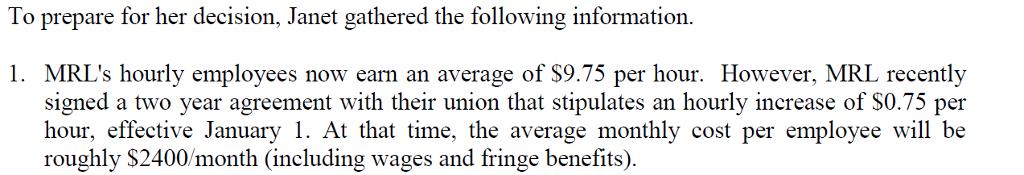
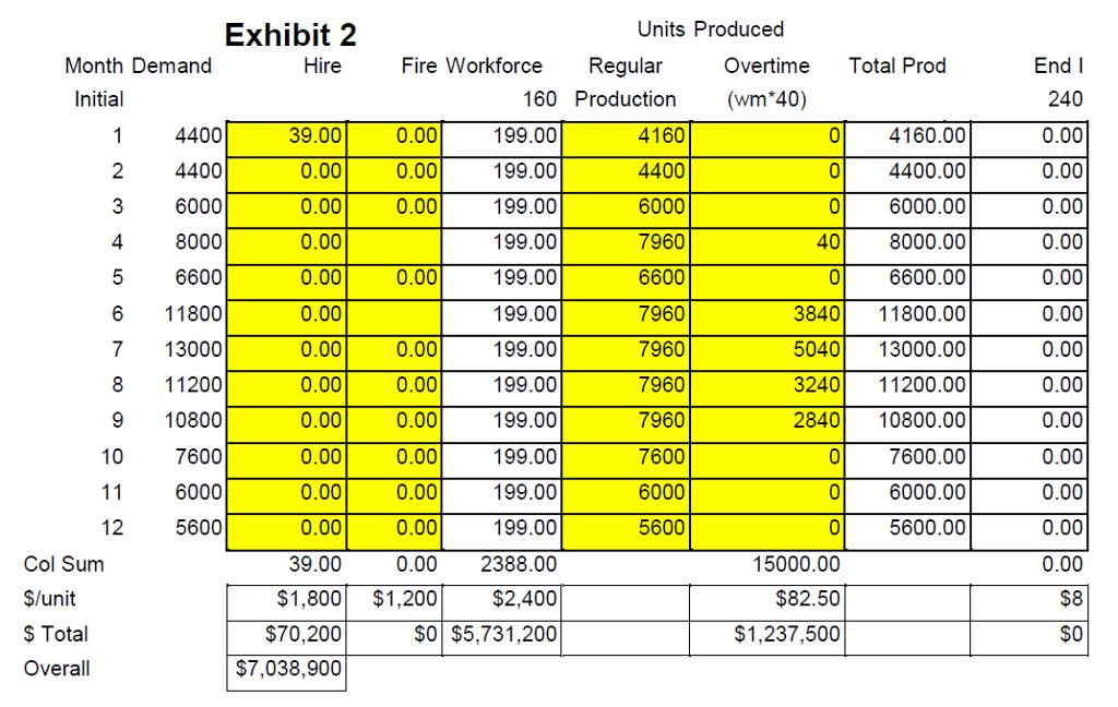
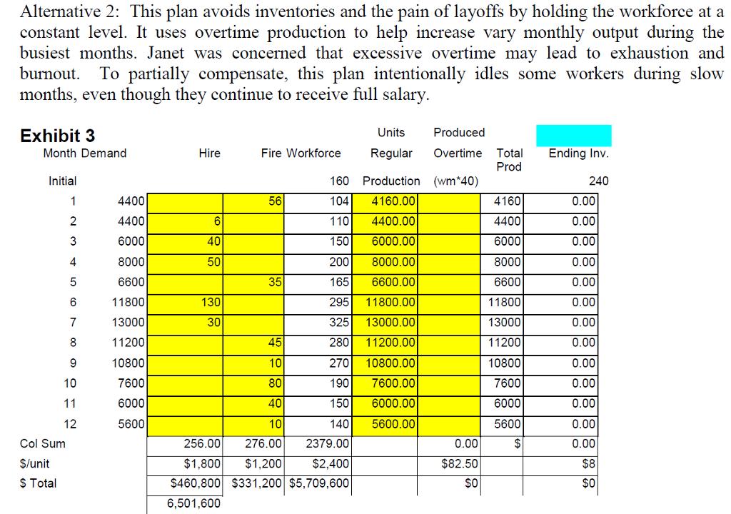
In early September Janet Huntley, the newly-appointed planner for MacDonald Refrigeration Ltd (MRL) of Sarnia, Ontario...

 

 
 
 
 

 
 
 
 
 
 
 
 
 

Transcribed Image Text:

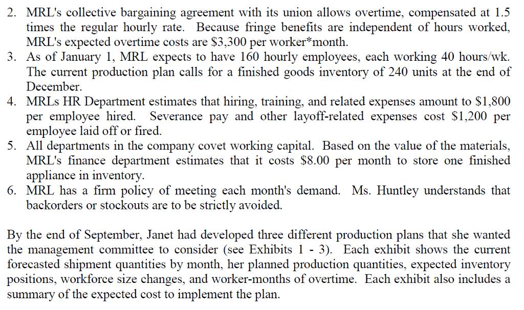
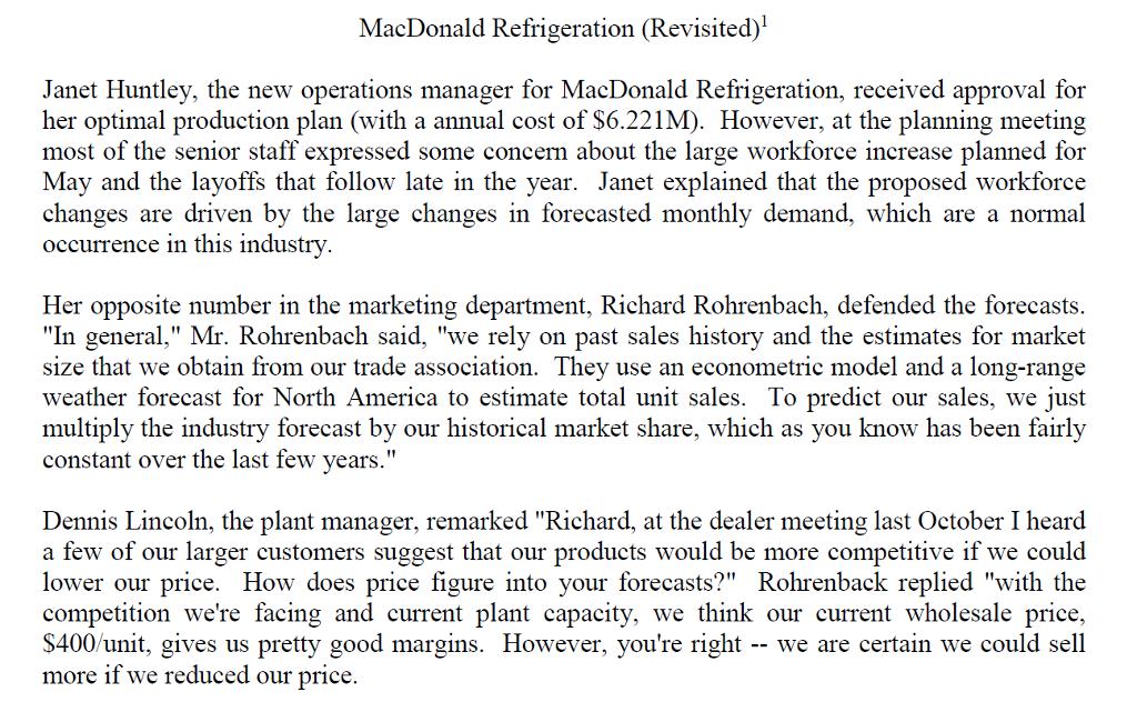
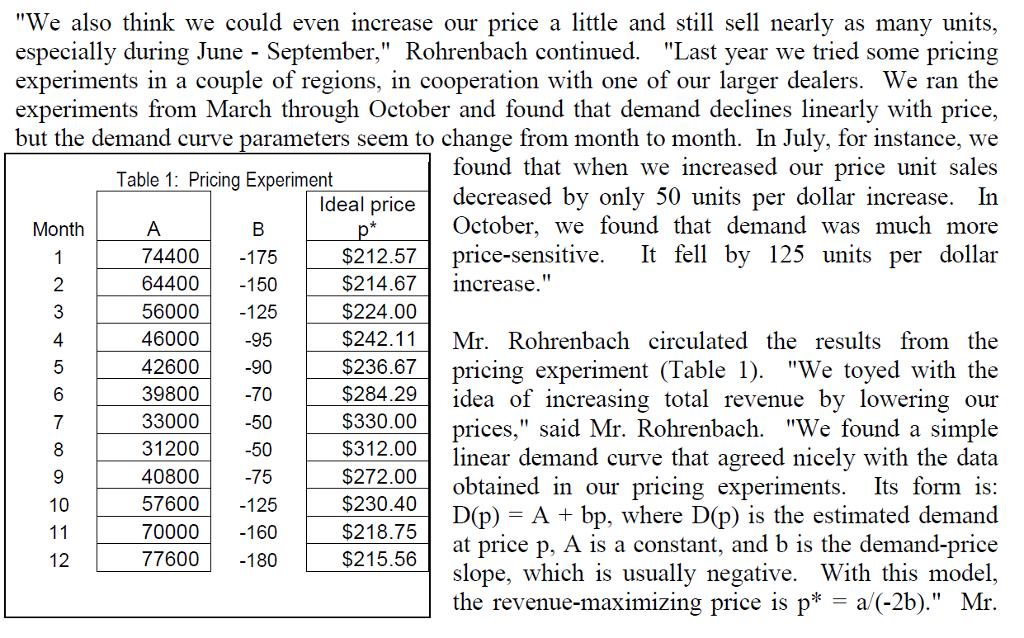
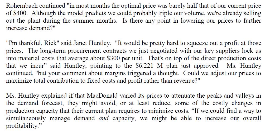
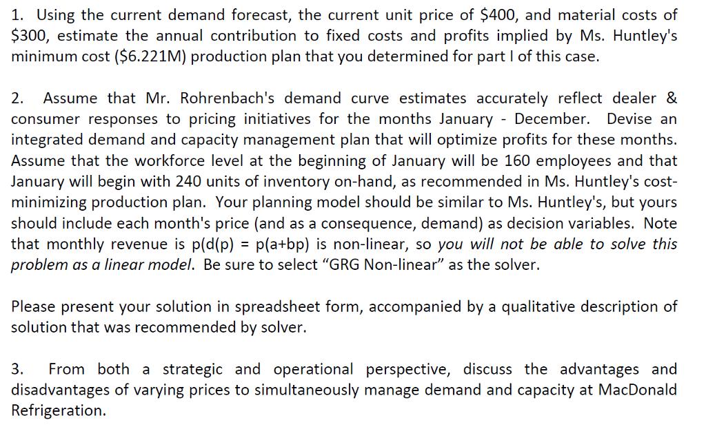
In early September Janet Huntley, the newly-appointed planner for MacDonald Refrigeration Ltd (MRL) of Sarnia, Ontario began working on MRLs production plan for the upcoming calendar year. The plan will be presented at MRLs regular management committee at the end of the month. BACKGROUND The company began operations near the Sarnia, Ontario airport in 1954 as manufacturer of commercial refrigeration systems. By 1987, MRL had diversified into consumer refrigeration and moved to a new 300,000 square foot manufacturing facility. Its current product line, consisting of commercial and residential air conditioning systems, refrigerators, and freezers, produced sales of $28.5 million last year. Through a combination of careful product design and investments in new process technology, MRL has seen the annual output per manufacturing employee increase from about 240 appliances in 1987 to an estimated 480 appliances next year. Their plant in Sarnia has the physical capacity to make up to 13,000 appliances per month. Although it varies by product type, typical throughput time is 3 days. THE PLANNING PROCESS Once each month, Ms. Huntley receives monthly sales forecasts updates for all of MRL appliances for 15 months into the future. Although the monthly forecasts are refined each month, MRL must order critical components about 3 months in advance of need. In effect, MRL commits its resources to the forecast no later than 3 months prior to the period when the sales are to take place. Due to the pronounced seasonality of refrigeration products, MRL develops production plans for 15 months into the future. However, with 90-day material lead times the first three months of the plan are effectively frozen; no longer subject to change. Therefore, the key portion of Ms. Huntley's plan will be the 12 month period that begins next January. Ms. Huntley's plan need not address specific models and sizes of appliances (those details are attended to when the detailed master schedule is created and updated). Instead, her production plan is a statement of how MRL will obtain sufficient capacity to build, in aggregate, the units they expect to sell during the coming year. Because the resource requirements for MRLs various products are roughly similar, Ms. Huntley's aggregate plan should be able to support a variety of different product mixes as long as the total production required is near the forecasted amount. prepare for her decision, Janet gathered the following information. 1. MRL's hourly employees now earn an average of $9.75 per hour. However, MRL recently signed a two year agreement with their union that stipulates an hourly increase of $0.75 per hour, effective January 1. At that time, the average monthly cost per employee will be roughly $2400/month (including wages and fringe benefits). To Month Demand Initial 1 2 3 4 5 6 7 8 9 10 11 12 Col Sum $/unit $ Total Overall 4400 4400 6000 8000 6600 11800 13000 11200 10800 7600 6000 5600 Exhibit 1 Hire Fire Workforce 160 51.00 0.00 211.00 0.00 0.00 211.00 0.00 0.00 211.00 0.00 0.00 211.00 0.00 0.00 211.00 0.00 0.00 211.00 0.00 0.00 211.00 0.00 0.00 211.00 0.00 0.00 211.00 0.00 0.00 211.00 0.00 0.00 211.00 0.00 0.00 211.00 51.00 0.00 2532.00 $1,800 $1,200 $2,400 $91,800 $0 $6,076,800 $6,768,600 Regular Overtime Total Production Prod. Prod 8440.00 8440.00 8440.00 8440.00 8440.00 8440.00 8440.00 8440.00 8440.00 8440.00 8440.00 8440.00 0.00 8440.00 0.00 8440.00 0.00 8440.00 0.00 8440.00 0.00 8440.00 0.00 8440.00 0.00 8440.00 0.00 8440.00 0.00 8440.00 0.00 8440.00 0.00 8440.00 0.00 8440.00 0.00 $82.50 $0 End Inv 240 4280.00 8320.00 10760.00 11200.00 13040.00 9680.00 5120.00 2360.00 0.00 840.00 3280.00 6120.00 75000.00 $8 $600,000 2. MRL's collective bargaining agreement with its union allows overtime, compensated at 1.5 times the regular hourly rate. Because fringe benefits are independent of hours worked, MRL's expected overtime costs are $3,300 per worker*month. 3. As of January 1, MRL expects to have 160 hourly employees, each working 40 hours/wk. The current production plan calls for a finished goods inventory of 240 units at the end of December. 4. MRLS HR Department estimates that hiring, training, and related expenses amount to $1,800 per employee hired. Severance pay and other layoff-related expenses cost $1,200 per employee laid off or fired. 5. All departments in the company covet working capital. Based on the value of the materials, MRL's finance department estimates that it costs $8.00 per month to store one finished appliance in inventory. 6. MRL has a firm policy of meeting each month's demand. Ms. Huntley understands that backorders or stockouts are to be strictly avoided. By the end of September, Janet had developed three different production plans that she wanted the management committee to consider (see Exhibits 1 - 3). Each exhibit shows the current forecasted shipment quantities by month, her planned production quantities, expected inventory positions, workforce size changes, and worker-months of overtime. Each exhibit also includes a summary of the expected cost to implement the plan. THE AGGREGATE PLANS Alternative 1: In this plan the monthly production quantity and the total number of employees remain constant throughout the year, at a level sufficient to meet peak demand. In periods of low demand inventories accumulate, and in months of high demand those inventories are drawn down. With ample inventories, this plan provides some protection against forecast errors. In addition, it does not stress the workforce with month after month of extensive overtime work. Month Demand Initial 1 2 3 4 5 6 11800 7 13000 8 11200 9 10800 10 11 12 4400 4400 6000 8000 6600 Col Sum $/unit $ Total Overall 7600 6000 5600 Exhibit 2 Hire 39.00 0.00 Fire Workforce 0.00 0.00 0.00 199.00 199.00 199.00 199.00 199.00 199.00 199.00 199.00 199.00 199.00 199.00 199.00 2388.00 $2,400 $0 $5,731,200 0.00 0.00 0.00 0.00 0.00 0.00 0.00 0.00 0.00 0.00 0.00 0.00 0.00 0.00 0.00 0.00 39.00 0.00 $1,800 $1,200 $70,200 $7,038,900 0.00 Units Produced Regular 160 Production 4160 4400 6000 7960 6600 7960 7960 7960 7960 7600 6000 5600 Overtime (wm*40) 0 0 0 40 0 4160.00 4400.00 6000.00 8000.00 6600.00 3840 11800.00 5040 13000.00 3240 11200.00 2840 10800.00 7600.00 6000.00 5600.00 0 0 0 Total Prod 15000.00 $82.50 $1,237,500 End I 240 0.00 0.00 0.00 0.00 0.00 0.00 0.00 0.00 0.00 0.00 0.00 0.00 0.00 $8 $0 Alternative 2: This plan avoids inventories and the pain of layoffs by holding the workforce at a constant level. It uses overtime production to help increase vary monthly output during the busiest months. Janet was concerned that excessive overtime may lead to exhaustion and burnout. To partially compensate, this plan intentionally idles some workers during slow months, even though they continue to receive full salary. Exhibit 3 Month Demand. Initial 1 2 3 4 5 6 7 8 9 10 11 12 Col Sum $/unit $ Total 4400 4400 6000 8000 6600 11800 13000 11200 10800 7600 6000 5600 Hire 6 40 50 130 30 Fire Workforce 56 35 45 10 80 40 10 160 104 110 150 200 165 Production (wm*40) 4160.00 4400.00 6000.00 8000.00 6600.00 295 11800.00 325 13000.00 280 11200.00 270 10800.00 190 7600.00 150 6000.00 140 5600.00 256.00 276.00 $1,800 $1,200 $460,800 $331,200 $5,709,600 6,501,600 2379.00 $2,400 Units Regular Produced Overtime Total Prod 0.00 $82.50 $0 4160 4400 6000 8000 6600 11800 13000 11200 10800 7600 6000 5600 $ Ending Inv. 240 0.00 0.00 0.00 0.00 0.00 0.00 0.00 0.00 0.00 0.00 0.00 0.00 0.00 $8 $0 Alternative 3: Janet's final plan overcomes some of the limitations of Alternative 2 by adjusting the size of the workforce in response to changing demand. Employee morale and union relations are likely to suffer under this plan, especially during the months with heavy layoffs. Those months calling for large numbers of new hires will not be stress free, since Sarnia's workforce is generally fully employed once the ice melts. While Janet's plans all seem to be feasible, she is not entirely happy with any of them. Among other things, she wonders whether there is a better (less costly) alternative for MRL. Part of the difficulty in developing these production plans is that they all must cope with extreme fluctuations in demand. Although Janet had no input in the forecasting process (MRL's marketing specialists are responsible for forecasting), she realizes that the forecasts are predicated on certain assumptions about price and product mix. She wonders whether different pricing and product mix decisions might take lead to forecasts with lower peaks and higher valleys. With more constant output requirements, she would have to make fewer and less extreme capacity changes. MacDonald Refrigeration (Revisited)¹ Janet Huntley, the new operations manager for MacDonald Refrigeration, received approval for her optimal production plan (with a annual cost of $6.221M). However, at the planning meeting most of the senior staff expressed some concern about the large workforce increase planned for May and the layoffs that follow late in the year. Janet explained that the proposed workforce changes are driven by the large changes in forecasted monthly demand, which are a normal occurrence in this industry. Her opposite number in the marketing department, Richard Rohrenbach, defended the forecasts. "In general," Mr. Rohrenbach said, "we rely on past sales history and the estimates for market size that we obtain from our trade association. They use an econometric model and a long-range weather forecast for North America to estimate total unit sales. To predict our sales, we just multiply the industry forecast by our historical market share, which as you know has been fairly constant over the last few years." Dennis Lincoln, the plant manager, remarked "Richard, at the dealer meeting last October I heard a few of our larger customers suggest that our products would be more competitive we could lower our price. How does price figure into your forecasts?" Rohrenback replied "with the competition we're facing and current plant capacity, we think our current wholesale price, $400/unit, gives us pretty good margins. However, you're right -- we are certain we could sell more if we reduced our price. "We also think we could even increase our price a little and still sell nearly as many units, especially during June - September," Rohrenbach continued. "Last year we tried some pricing experiments in a couple of regions, in cooperation with one of our larger dealers. We ran the experiments from March through October and found that demand declines linearly with price, but the demand curve parameters seem to change from month to month. In July, for instance, we Table 1: Pricing Experiment found that when we increased our price unit sales decreased by only 50 units per dollar increase. In October, we found that demand was much more price-sensitive. It fell by 125 units per dollar increase." Month 1 NT600 W N 3 4 5 6 7 8 9 10 11 12 B A 74400 -175 64400 -150 56000 -125 46000 -95 42600 -90 39800 -70 -50 33000 31200 -50 40800 -75 57600 -125 70000 -160 77600 -180 Ideal price p* $212.57 $214.67 $224.00 $242.11 $236.67 $284.29 $330.00 $312.00 $272.00 $230.40 $218.75 $215.56 Mr. Rohrenbach circulated the results from the pricing experiment (Table 1). "We toyed with the idea of increasing total revenue by lowering our prices," said Mr. Rohrenbach. "We found a simple linear demand curve that agreed nicely with the data obtained in our pricing experiments. Its form is: D(p) A+bp, where D(p) is the estimated demand at price p, A is a constant, and b is the demand-price slope, which is usually negative. With this model, the revenue-maximizing price is p* = a/(-2b)." Mr. Rohernbach continued "in most months the optimal price was barely half that of our current price of $400. Although the model predicts we could probably triple our volume, we're already selling out the plant during the summer months. Is there any point in lowering our prices to further increase demand?" "I'm thankful, Rick" said Janet Huntley. "It would be pretty hard to squeeze out a profit at those prices. The long-term procurement contracts we just negotiated with our key suppliers lock us into material costs that average about $300 per unit. That's on top of the direct production costs that we incur" said Huntley, pointing to the $6.221 M plan just approved. Ms. Huntley continued, "but your comment about margins triggered a thought. Could we adjust our prices to maximize total contribution to fixed costs and profit rather than revenue?" Ms. Huntley explained if that MacDonald varied its prices to attenuate the peaks and valleys in the demand forecast, they might avoid, or at least reduce, some of the costly changes in production capacity that their current plan requires to minimize costs. "If we could find a way to simultaneously manage demand and capacity, we might be able to increase our overall profitability." 1. Using the current demand forecast, the current unit price of $400, and material costs of $300, estimate the annual contribution to fixed costs and profits implied by Ms. Huntley's minimum cost ($6.221M) production plan that you determined for part I of this case. 2. Assume that Mr. Rohrenbach's demand curve estimates accurately reflect dealer & consumer responses to pricing initiatives for the months January December. Devise an integrated demand and capacity management plan that will optimize profits for these months. Assume that the workforce level at the beginning of January will be 160 employees and that January will begin with 240 units of inventory on-hand, as recommended in Ms. Huntley's cost- minimizing production plan. Your planning model should be similar to Ms. Huntley's, but yours should include each month's price (and as a consequence, demand) as decision variables. Note that monthly revenue is p(d(p) = p(a+bp) is non-linear, so you will not be able to solve this problem as a linear model. Be sure to select "GRG Non-linear" as the solver. Please present your solution in spreadsheet form, accompanied by a qualitative description of solution that was recommended by solver. 3. From both a strategic and operational perspective, discuss the advantages and disadvantages of varying prices to simultaneously manage demand and capacity at MacDonald Refrigeration. In early September Janet Huntley, the newly-appointed planner for MacDonald Refrigeration Ltd (MRL) of Sarnia, Ontario began working on MRLs production plan for the upcoming calendar year. The plan will be presented at MRLs regular management committee at the end of the month. BACKGROUND The company began operations near the Sarnia, Ontario airport in 1954 as manufacturer of commercial refrigeration systems. By 1987, MRL had diversified into consumer refrigeration and moved to a new 300,000 square foot manufacturing facility. Its current product line, consisting of commercial and residential air conditioning systems, refrigerators, and freezers, produced sales of $28.5 million last year. Through a combination of careful product design and investments in new process technology, MRL has seen the annual output per manufacturing employee increase from about 240 appliances in 1987 to an estimated 480 appliances next year. Their plant in Sarnia has the physical capacity to make up to 13,000 appliances per month. Although it varies by product type, typical throughput time is 3 days. THE PLANNING PROCESS Once each month, Ms. Huntley receives monthly sales forecasts updates for all of MRL appliances for 15 months into the future. Although the monthly forecasts are refined each month, MRL must order critical components about 3 months in advance of need. In effect, MRL commits its resources to the forecast no later than 3 months prior to the period when the sales are to take place. Due to the pronounced seasonality of refrigeration products, MRL develops production plans for 15 months into the future. However, with 90-day material lead times the first three months of the plan are effectively frozen; no longer subject to change. Therefore, the key portion of Ms. Huntley's plan will be the 12 month period that begins next January. Ms. Huntley's plan need not address specific models and sizes of appliances (those details are attended to when the detailed master schedule is created and updated). Instead, her production plan is a statement of how MRL will obtain sufficient capacity to build, in aggregate, the units they expect to sell during the coming year. Because the resource requirements for MRLs various products are roughly similar, Ms. Huntley's aggregate plan should be able to support a variety of different product mixes as long as the total production required is near the forecasted amount. prepare for her decision, Janet gathered the following information. 1. MRL's hourly employees now earn an average of $9.75 per hour. However, MRL recently signed a two year agreement with their union that stipulates an hourly increase of $0.75 per hour, effective January 1. At that time, the average monthly cost per employee will be roughly $2400/month (including wages and fringe benefits). To Month Demand Initial 1 2 3 4 5 6 7 8 9 10 11 12 Col Sum $/unit $ Total Overall 4400 4400 6000 8000 6600 11800 13000 11200 10800 7600 6000 5600 Exhibit 1 Hire Fire Workforce 160 51.00 0.00 211.00 0.00 0.00 211.00 0.00 0.00 211.00 0.00 0.00 211.00 0.00 0.00 211.00 0.00 0.00 211.00 0.00 0.00 211.00 0.00 0.00 211.00 0.00 0.00 211.00 0.00 0.00 211.00 0.00 0.00 211.00 0.00 0.00 211.00 51.00 0.00 2532.00 $1,800 $1,200 $2,400 $91,800 $0 $6,076,800 $6,768,600 Regular Overtime Total Production Prod. Prod 8440.00 8440.00 8440.00 8440.00 8440.00 8440.00 8440.00 8440.00 8440.00 8440.00 8440.00 8440.00 0.00 8440.00 0.00 8440.00 0.00 8440.00 0.00 8440.00 0.00 8440.00 0.00 8440.00 0.00 8440.00 0.00 8440.00 0.00 8440.00 0.00 8440.00 0.00 8440.00 0.00 8440.00 0.00 $82.50 $0 End Inv 240 4280.00 8320.00 10760.00 11200.00 13040.00 9680.00 5120.00 2360.00 0.00 840.00 3280.00 6120.00 75000.00 $8 $600,000 2. MRL's collective bargaining agreement with its union allows overtime, compensated at 1.5 times the regular hourly rate. Because fringe benefits are independent of hours worked, MRL's expected overtime costs are $3,300 per worker*month. 3. As of January 1, MRL expects to have 160 hourly employees, each working 40 hours/wk. The current production plan calls for a finished goods inventory of 240 units at the end of December. 4. MRLS HR Department estimates that hiring, training, and related expenses amount to $1,800 per employee hired. Severance pay and other layoff-related expenses cost $1,200 per employee laid off or fired. 5. All departments in the company covet working capital. Based on the value of the materials, MRL's finance department estimates that it costs $8.00 per month to store one finished appliance in inventory. 6. MRL has a firm policy of meeting each month's demand. Ms. Huntley understands that backorders or stockouts are to be strictly avoided. By the end of September, Janet had developed three different production plans that she wanted the management committee to consider (see Exhibits 1 - 3). Each exhibit shows the current forecasted shipment quantities by month, her planned production quantities, expected inventory positions, workforce size changes, and worker-months of overtime. Each exhibit also includes a summary of the expected cost to implement the plan. THE AGGREGATE PLANS Alternative 1: In this plan the monthly production quantity and the total number of employees remain constant throughout the year, at a level sufficient to meet peak demand. In periods of low demand inventories accumulate, and in months of high demand those inventories are drawn down. With ample inventories, this plan provides some protection against forecast errors. In addition, it does not stress the workforce with month after month of extensive overtime work. Month Demand Initial 1 2 3 4 5 6 11800 7 13000 8 11200 9 10800 10 11 12 4400 4400 6000 8000 6600 Col Sum $/unit $ Total Overall 7600 6000 5600 Exhibit 2 Hire 39.00 0.00 Fire Workforce 0.00 0.00 0.00 199.00 199.00 199.00 199.00 199.00 199.00 199.00 199.00 199.00 199.00 199.00 199.00 2388.00 $2,400 $0 $5,731,200 0.00 0.00 0.00 0.00 0.00 0.00 0.00 0.00 0.00 0.00 0.00 0.00 0.00 0.00 0.00 0.00 39.00 0.00 $1,800 $1,200 $70,200 $7,038,900 0.00 Units Produced Regular 160 Production 4160 4400 6000 7960 6600 7960 7960 7960 7960 7600 6000 5600 Overtime (wm*40) 0 0 0 40 0 4160.00 4400.00 6000.00 8000.00 6600.00 3840 11800.00 5040 13000.00 3240 11200.00 2840 10800.00 7600.00 6000.00 5600.00 0 0 0 Total Prod 15000.00 $82.50 $1,237,500 End I 240 0.00 0.00 0.00 0.00 0.00 0.00 0.00 0.00 0.00 0.00 0.00 0.00 0.00 $8 $0 Alternative 2: This plan avoids inventories and the pain of layoffs by holding the workforce at a constant level. It uses overtime production to help increase vary monthly output during the busiest months. Janet was concerned that excessive overtime may lead to exhaustion and burnout. To partially compensate, this plan intentionally idles some workers during slow months, even though they continue to receive full salary. Exhibit 3 Month Demand. Initial 1 2 3 4 5 6 7 8 9 10 11 12 Col Sum $/unit $ Total 4400 4400 6000 8000 6600 11800 13000 11200 10800 7600 6000 5600 Hire 6 40 50 130 30 Fire Workforce 56 35 45 10 80 40 10 160 104 110 150 200 165 Production (wm*40) 4160.00 4400.00 6000.00 8000.00 6600.00 295 11800.00 325 13000.00 280 11200.00 270 10800.00 190 7600.00 150 6000.00 140 5600.00 256.00 276.00 $1,800 $1,200 $460,800 $331,200 $5,709,600 6,501,600 2379.00 $2,400 Units Regular Produced Overtime Total Prod 0.00 $82.50 $0 4160 4400 6000 8000 6600 11800 13000 11200 10800 7600 6000 5600 $ Ending Inv. 240 0.00 0.00 0.00 0.00 0.00 0.00 0.00 0.00 0.00 0.00 0.00 0.00 0.00 $8 $0 Alternative 3: Janet's final plan overcomes some of the limitations of Alternative 2 by adjusting the size of the workforce in response to changing demand. Employee morale and union relations are likely to suffer under this plan, especially during the months with heavy layoffs. Those months calling for large numbers of new hires will not be stress free, since Sarnia's workforce is generally fully employed once the ice melts. While Janet's plans all seem to be feasible, she is not entirely happy with any of them. Among other things, she wonders whether there is a better (less costly) alternative for MRL. Part of the difficulty in developing these production plans is that they all must cope with extreme fluctuations in demand. Although Janet had no input in the forecasting process (MRL's marketing specialists are responsible for forecasting), she realizes that the forecasts are predicated on certain assumptions about price and product mix. She wonders whether different pricing and product mix decisions might take lead to forecasts with lower peaks and higher valleys. With more constant output requirements, she would have to make fewer and less extreme capacity changes. MacDonald Refrigeration (Revisited)¹ Janet Huntley, the new operations manager for MacDonald Refrigeration, received approval for her optimal production plan (with a annual cost of $6.221M). However, at the planning meeting most of the senior staff expressed some concern about the large workforce increase planned for May and the layoffs that follow late in the year. Janet explained that the proposed workforce changes are driven by the large changes in forecasted monthly demand, which are a normal occurrence in this industry. Her opposite number in the marketing department, Richard Rohrenbach, defended the forecasts. "In general," Mr. Rohrenbach said, "we rely on past sales history and the estimates for market size that we obtain from our trade association. They use an econometric model and a long-range weather forecast for North America to estimate total unit sales. To predict our sales, we just multiply the industry forecast by our historical market share, which as you know has been fairly constant over the last few years." Dennis Lincoln, the plant manager, remarked "Richard, at the dealer meeting last October I heard a few of our larger customers suggest that our products would be more competitive we could lower our price. How does price figure into your forecasts?" Rohrenback replied "with the competition we're facing and current plant capacity, we think our current wholesale price, $400/unit, gives us pretty good margins. However, you're right -- we are certain we could sell more if we reduced our price. "We also think we could even increase our price a little and still sell nearly as many units, especially during June - September," Rohrenbach continued. "Last year we tried some pricing experiments in a couple of regions, in cooperation with one of our larger dealers. We ran the experiments from March through October and found that demand declines linearly with price, but the demand curve parameters seem to change from month to month. In July, for instance, we Table 1: Pricing Experiment found that when we increased our price unit sales decreased by only 50 units per dollar increase. In October, we found that demand was much more price-sensitive. It fell by 125 units per dollar increase." Month 1 NT600 W N 3 4 5 6 7 8 9 10 11 12 B A 74400 -175 64400 -150 56000 -125 46000 -95 42600 -90 39800 -70 -50 33000 31200 -50 40800 -75 57600 -125 70000 -160 77600 -180 Ideal price p* $212.57 $214.67 $224.00 $242.11 $236.67 $284.29 $330.00 $312.00 $272.00 $230.40 $218.75 $215.56 Mr. Rohrenbach circulated the results from the pricing experiment (Table 1). "We toyed with the idea of increasing total revenue by lowering our prices," said Mr. Rohrenbach. "We found a simple linear demand curve that agreed nicely with the data obtained in our pricing experiments. Its form is: D(p) A+bp, where D(p) is the estimated demand at price p, A is a constant, and b is the demand-price slope, which is usually negative. With this model, the revenue-maximizing price is p* = a/(-2b)." Mr. Rohernbach continued "in most months the optimal price was barely half that of our current price of $400. Although the model predicts we could probably triple our volume, we're already selling out the plant during the summer months. Is there any point in lowering our prices to further increase demand?" "I'm thankful, Rick" said Janet Huntley. "It would be pretty hard to squeeze out a profit at those prices. The long-term procurement contracts we just negotiated with our key suppliers lock us into material costs that average about $300 per unit. That's on top of the direct production costs that we incur" said Huntley, pointing to the $6.221 M plan just approved. Ms. Huntley continued, "but your comment about margins triggered a thought. Could we adjust our prices to maximize total contribution to fixed costs and profit rather than revenue?" Ms. Huntley explained if that MacDonald varied its prices to attenuate the peaks and valleys in the demand forecast, they might avoid, or at least reduce, some of the costly changes in production capacity that their current plan requires to minimize costs. "If we could find a way to simultaneously manage demand and capacity, we might be able to increase our overall profitability." 1. Using the current demand forecast, the current unit price of $400, and material costs of $300, estimate the annual contribution to fixed costs and profits implied by Ms. Huntley's minimum cost ($6.221M) production plan that you determined for part I of this case. 2. Assume that Mr. Rohrenbach's demand curve estimates accurately reflect dealer & consumer responses to pricing initiatives for the months January December. Devise an integrated demand and capacity management plan that will optimize profits for these months. Assume that the workforce level at the beginning of January will be 160 employees and that January will begin with 240 units of inventory on-hand, as recommended in Ms. Huntley's cost- minimizing production plan. Your planning model should be similar to Ms. Huntley's, but yours should include each month's price (and as a consequence, demand) as decision variables. Note that monthly revenue is p(d(p) = p(a+bp) is non-linear, so you will not be able to solve this problem as a linear model. Be sure to select "GRG Non-linear" as the solver. Please present your solution in spreadsheet form, accompanied by a qualitative description of solution that was recommended by solver. 3. From both a strategic and operational perspective, discuss the advantages and disadvantages of varying prices to simultaneously manage demand and capacity at MacDonald Refrigeration.

Answer rating: 100% (QA)

MacDonald Refrigeration Ltd MRL is a company that has been in business since 1954 and is located near the Sarnia Ontario airport The company specializ... View the full answer