

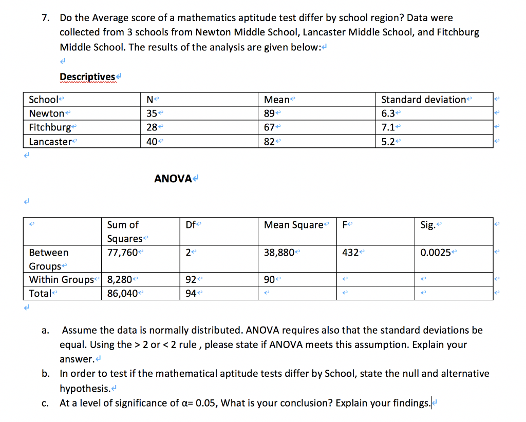
J d 7. Do the Average score of a mathematics aptitude test differ by school region?...
Fantastic news! We've Found the answer you've been seeking!
Question:

Transcribed Image Text:
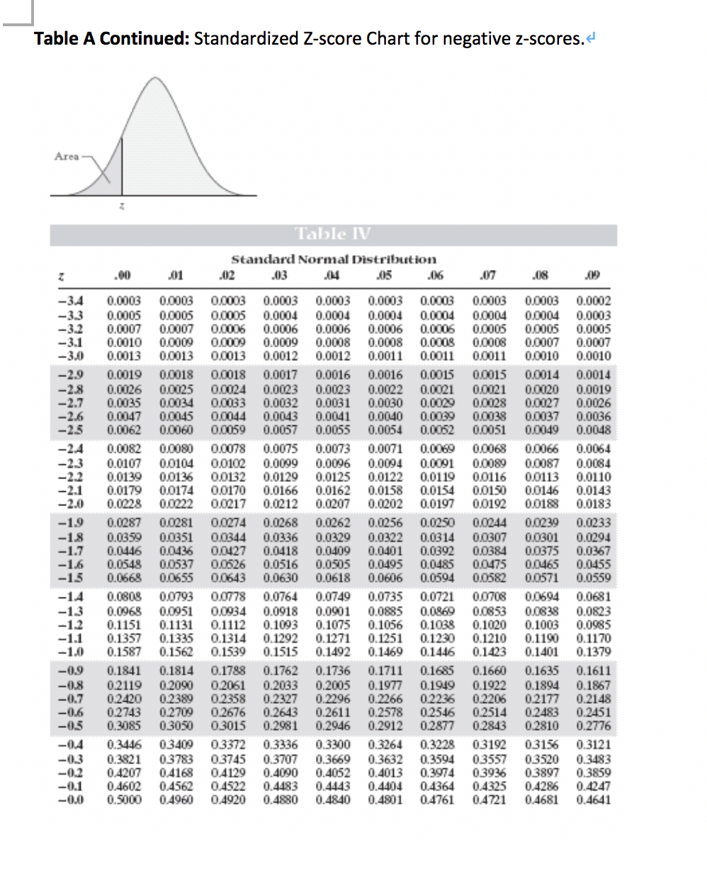
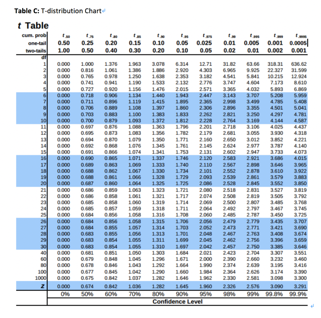
J d 7. Do the Average score of a mathematics aptitude test differ by school region? Data were collected from 3 schools from Newton Middle School, Lancaster Middle School, and Fitchburg Middle School. The results of the analysis are given below: < School Newton Fitchburg Lancaster J J Descriptives < Between Groups Within Groups Total a. Sum of Squares 77,760* 8,280* 86,040* Ne 35* 28 40* ANOVA < Df 2 92* 94 < Mean 89* 67 82 Mean Square* 38,880* 90* e F 432* e e Standard deviation 6.3 7.1 5.2 Sig. 0.0025* e Assume the data is normally distributed. ANOVA requires also that the standard deviations be equal. Using the > 2 or < 2 rule, please state if ANOVA meets this assumption. Explain your answer. < b. In order to test if the mathematical aptitude tests differ by School, state the null and alternative hypothesis. < C. At a level of significance of a= 0.05, What is your conclusion? Explain your findings. P Table A: Standardized z-score chart for positive z-scores < STANDARD STATISTICAL TABLES 1. Areas under the Normal Distribution The table gives the cumulative probability up to the standardised normal value z i.e. 2 P[ Z < 2 ] Z CEEEE EEEE! 88::: ::::: 0.0 0.5000 0.1 0.5398 0.2 0.5793 0.3 0.6179 0.6554 0.4 0.5 0.6 0.7 0.8 0.9 1.0 1.1 1.2 1.3 1.4 1.5 1.6 1.7 1.8 0.00 1.9 -0 1 exp(-2) dz 27 0.01 0.02 0.03 0.04 0.05 0.06 0.07 0.5040 0.5080 0.5120 0.5159 0.5438 0.5478 0.5517 0.5557 0.5832 0.5871 0.5910 0.5948 0.6217 0.6255 0.6293 0.6331 0.6591 0.6628 0.6664 0.8413 0.8438 0.8461 0.8643 0.8665 0.8686 0.8849 0.8869 0.8888 0.9032 0.9049 0.9066 0.9192 0.9207 0.9222 0 0.8485 0.8508 0.8708 0.8729 0.8907 0.8925 0.9082 0.9099 0.9236 0.9251 P[ Z < Z ] 0.9382 9332 0.9345 0.9357 0.931 0.9452 0.9463 0.9474 0.9484 0.9495 0.9554 0.9564 0.9573 0.9582 0.9591 0.9641 0.9649 0.9656 0.9664 0.9671 0.9713 0.9719 0.9726 0.9732 0.9738 Z 0.08 0.5199 0.5596 0.5987 0.6026 0.6064 0.6103 0.6368 0.6406 0.6443 0.6480 0.6700 0.6736 0.6772 0.6808 0.6844 0.6915 0.6950 0.6985 0.7019 0.7054 0.7257 0.7291 0.7324 0.7357 0.7389 0.7580 0.7611 0.7642 0.7673 0.7704 0.7734 0.7764 0.7794 0.7823 0.7881 0.7910 0.7939 0.7967 0.7995 0.8023 0.8051 0.8159 0.8186 0.8212 0.8238 0.8264 0.8289 0.8315 0.8078 0.8106 0.8340 0.8365 0.5239 0.5279 0.5319 0.5359 0.5636 0.5675 0.5714 0.5753 0.7088 0.7123 0.7157 0.7190 0.7224 0.7422 0.7454 0.7486 0.7517 0.7549 0.7854 0.8531 0.8554 0.8577 0.8599 0.8749 0.8770 0.8790 0.8804 0.8944 0.8962 0.8980 0.8997 0.9147 0.9162 0.9115 0.9131 0.9265 0.9279 0.9292 0.9306 9394 9406 0.9505 0.9515 0.9599 0.9608 0.9678 0.9686 0.9693 0.9699 0.9744 0.9750 0.9756 0.9761 9418 0.9 0.09 0.9525 0.9535 0.9616 0.9625 0.6141 0.6517 0.6879 0.8133 0.8389 0.8621 0.8830 0.9015 0.9177 0.9319 0.9441 0.9545 0.9633 0.9706 0.9767 2.0 0.9773 0.9778 0.9783 0.9788 0.9793 2.1 0.9821 0.9826 0.9830 0.9834 0.9838 2.2 0.9861 0.9865 0.9868 0.9871 2.3 0.9893 0.9896 0.9898 0.9901 2.4 0.9918 0.9920 0.9922 0.9924 0.9798 0.9803 0.9808 0.9812 0.9817 0.9842 0.9846 0.9850 0.9854 0.9857 0.9874 0.9878 0.9881 0.9884 0.9887 0.9904 0.9906 0.9909 0.9911 0.9913 0.9931 0.9932 0.9934 0.9927 0.9929 NNNNN 0.9945 0.9946 2.5 0.9938 0.9940 0.9941 0.9943 0.9948 0.9949 0.9951 0.9952 2.6 0.9953 0.9955 0.9956 0.9957 0.9959 0.9960 0.9961 0.9962 0.9963 0.9964 2.7 0.9965 0.9966 0.9967 0.9968 0.9969 0.9970 0.9971 0.9972 0.9973 0.9974 2.8 0.9974 0.9975 0.9976 0.9977 0.9977 0.9978 0.9979 0.9980 0.9980 0.9981 2.9 0.9981 0.9982 0.9982 0.9983 0.9984 0.9984 0.9985 0.9985 0.9986 0.9986 2 P 0.9890 0.9916 0.9936 3.00 3.10 3.20 3.30 3.40 3.50 3.60 3.70 3.80 3.90 0.9986 0.9990 0.9993 0.9995 0.9997 0.9998 0.9998 0.9999 0.9999 1.0000 df 1 2 3 5 6 7 8 9 10 11 12 13 12245 X305 0.000 0.010 0.072 0.207 0412 0.676 0.989 1344 1.735 2.156 2.603 3.074 3.565 4.075 4.601 16 5.142 17 5.697 18 6.265 19 6844 20 7.434 X300 0.000 0.020 0.115 0.297 0.554 0.872 1.239 1.646 2.088 2.558 3.053 3.571 4.107 4.660 5.229 5.812 6.408 7.015 7.633 8.260 Chi-Square Distribution Table The shaded area is equal to a for x = x. X-975 0.001 0.051 0.216 0.484 0.831 1.237 1.690 2.180 2.700 3.247 3.816 4.404 5.009 5.629 6.262 6.908 7.564 0 8.231 8.907 9.591 X-950 0.004 0.103 0.352 0.711 1.145 1.635 2.167 2.733 3.325 3.940 4.575 5.226 5.892 X3900 0.016 0.211 0.584 1.064 1.610 2.204 2.833 3.490 4.168 4.865 5.578 6.304 7.042 X100 X050 2.706 3.841 4.605 5.991 6.251 7.815 9.348 11.345 7.779 9.488 11.143 13.277 9.236 11.070 12.833 15.086 10.645 14.449 12.592 14.067 16.013 12.017 13.362 15.507 14.684 16.919 15.987 18.307 19.675 18.549 21.026 17.275 19.812 22.362 7.790 8.547 6.571 7.261 7.962 8.672 9.390 10.865 25.989 11.651 27.204 10.117 10851 12.443 28.412 X025 5.024 7.378 21.064 26.119 23.685 22.307 24.996 27.488 9.312 23.542 10.085 24.769 X010 6.635 9.210 28.845 26.296 27.587 30.191 28.869 31.526 30.144 32.852 31.410 34.170 16812 18.475 17.535 20.090 23.589 19.023 21.666 20.483 23.209 21.920 24.725 25.188 26.757 23.337 26.217 28.300 24.736 27.688 29.819 31.319 32.801 29.141 30.578 005 32.000 33.409 7.879 10.597 12.838 14.860 16.750 18.548 20.278 21.955 34.267 35.718 34.805 37.156 36.191 38.582 37.566 39.997 35.172 38.076 8.897 10.283 11.591 9.542 10.982 12.338 10.196 11.689 13.091 10.856 12.401 13848 13.120 14.611 15.379 13.240 29.615 32.671 14.041 30.813 14.848 32.007 15.659 33.196 36.415 16.473 34.382 37.652 38.885 40.113 43.195 10.520 11.524 17.292 27 12.198 13.844 11.808 12.879 14.573 16.151 15.308 16.928 18.939 18.114 28 12.461 13.565 41.337 44.461 29 17.708 19.768 30 18.493 20.599 24.433 26.509 29.051 40 20.707 22.164 50 27.991 29.707 32.357 34.764 35.534 37.485 40.482 43.188 43.275 45.442 48.758 51.739 55.329 51.172 53.540 57.153 60.391 64.278 37.689 46.459 74.397 60 85.527 96.578 73.291 107.565 113.145 118.136 124.116 82.358 118.498 124.342 129.561 135.807 21 8.034 22 8.643 23 9.260 24 9.886 25 26 11.160 70 80 13.121 13.787 14.256 16.047 14.953 16.791 90 59.196 61.754 65.647 100 67.328 70.065 74.222 69.126 77.929 36.741 37.916 39.087 40.256 35.479 38.932 41.401 33.924 36.781 40.289 42.796 41.638 44.181 39.364 42.980 45.559 40.646 44314 46.928 41.923 45.642 48.290 46.963 48.278 42.557 45.722 49.588 43.773 46.979 50.892 59.342 63.691 76.154 83.298 88.379 95.023 100.425 106.629 112.329 51.805 55.758 63.167 67.505 71.420 79.082 90.531 101 879 49.645 50.993 52.336 53.672 66.766 79.490 91.952 104.215 116.321 128.299 140.169 Table A Continued: Standardized Z-score Chart for negative z-scores. < Area- Table IV Standard Normal Distribution .03 04 .05 z .00 .01 .02 .06 .07 .08 -3.4 0.0003 0.0003 0.0003 0.0003 0.0003 0.0003 0.0003 0.0003 0.0003 0.0002 -3.3 0.0005 0.0005 0.0005 0.0004 0.0004 0.0004 0.0004 0.0004 0.0004 0.0003 -3.2 0.0007 0.0007 0.0006 0.0006 0.0006 0.0006 0.0006 0.0005 0.0005 0.0005 -3.1 0.0010 0.0009 0.0009 0.0009 0.0008 0.0008 0.0008 0.0008 0.0007 0.0007 -3.0 0.0013 0.0013 0.0013 0.0012 0.0012 0.0011 0.0011 0.0011 0.0010 0.0010 -2.9 0.0019 0.0018 0.0018 0.0017 0.0016 0.0016 0.0015 0.0015 0.0014 0.0014 -2.8 0.0026 0.0025 0.0024 0.0023 0.0023 0.0022 0.0021 0.0021 0.0020 0.0019 -2.7 0.0035 0.0034 0.0033 0.0032 0.0031 0.0030 0.0029 0.0028 0.0027 0.0026 -2.6 0.0047 0.0045 0.0044 0.0043 0.0041 0.0040 0.0039 0.0038 0.0037 0.0036 -2.5 0.0062 0.0060 0.0059 0.0057 0.0055 0.0054 0.0052 0.0051 0.0049 0.0048 -2.4 0.0082 0.0080 0.0078 0.0075 0.0073 0.0071 0.0069 0.0068 0.0066 -2.3 0.0107 0.0104 0.0102 0.0099 0.0096 0.0094 0.0091 0.0089 0.0087 -2.2 0.0139 0.0136 0.0132 0.0129 0.0125 0.0122 0.0119 0.0116 0.0113 0.0110 -2.1 0.0179 0.0174 0.0170 0.0166 0.0162 0.0158 0.0154 0.0150 0.0146 0.0143 -2.0 0.0228 0.0222 0.0217 0.0212 0.0207 0.0202 0.0197 0.0192 0.0188 0.0183 0.0262 0.0256 0.0250 0.0329 0.0064 0.0084 -1.9 0.0287 0.0244 0.0239 0.0281 0.0274 0.0268 0.0336 -1.8 0.0359 0.0351 0.0344 0.0322 0.0314 0.0307 0.0301 0.1190 0.1170 -1.0 0.1401 0.1379 0.1635 0.1611 -1.7 0.0446 0.0436 0.0427 0.0418 0.0409 0.0401 0.0392 0.0384 0.0375 -1.6 0.0548 0.0537 0.0526 0.0516 0.0505 0.0495 0.0485 0.0475 0.0465 -1.5 0.0668 0.0655 0.0643 0.0630 0.0618 0.0606 0.0594 0.0582 0.0571 -1.4 0.0808 0.0793 0.0778 0.0764 0.0749 0.0735 0.0721 0.0708 0.0694 0.0681 -1.3 0.0968 0.0951 0.0934 0.0918 0.0901 0.0885 0.0869 0.0853 0.0838 0.0823 -1.2 0.1151 0.1131 0.1112 0.1093 0.1075 0.1056 0.1038 0.1020 0.1003 0.0985 -1.1 0.1357 0.1335 0.1314 0.1292 0.1271 0.1251 0.1230 0.1210 0.1587 0.1562 0.1539 0.1515 0.1492 0.1469 0.1446 0.1423 -0.9 0.1841 0.1814 0.1788 0.1762 0.1736 0.1711 0.1685 0.1660 -0.8 0.2119 0.2090 0.2061 0.2033 0.2005 0.1977 0.1949 0.1922 0.1894 0.1867 -0.7 0.2420 0.2389 0.2358 0.2327 0.2296 0.2266 0.2236 0.2206 0.2177 0.2148 -0.6 0.2743 0.2709 0.2676 0.2643 0.2611 0.2578 0.2546 0.2514 0.2483 0.2451 -0.5 0.3085 03050 0.3015 0.2981 0.2946 0.2912 0.2877 0.2843 0.2810 0.2776 -0.4 0.3446 03409 03372 0.3336 0.3300 0.3264 0.3228 03192 0.3156 0.3121 -0.3 0.3821 03783 03745 0.3707 0.3669 0.3632 0.3594 0.3557 03520 0.3483 -0.2 0.4207 0.4168 0.4129 0.4090 0.4052 0.4013 0.3974 0.3936 03897 0.3859 -0.1 0.4602 0.4562 0,4522 0.4483 0.4443 0.4404 0.4364 0.4325 0.4286 0.4247 -0.0 0.5000 0.4960 0.4920 0.4880 0.4840 0.4761 0.4721 0.4681 0.4641 0.4801 09 0.0233 0.0294 0.0367 0.0455 0.0559 Table C: T-distribution Chart t Table cum. prob one-tail two-tails df 1 2 3 4 5 6 7 8 9 10 11 12 13 14 15 16 17 18 19 20 21 22 23 24 25 t.75 t so 0.50 0.25 1.00 0.50 1.000 1.376 1.963 3.078 6.314 12.71 31.82 63.66 318.31 6.965 9.925 22.327 0.816 1.061 0.765 0.978 0.741 7.173 0.000 0.727 1.386 1.886 2.920 4.303 1.250 1.638 2.353 3.182 4.541 5.841 10.215 0.941 1.190 1.533 2.132 2.776 3.747 4.604 1.476 2.015 2.571 3.365 1.440 1.943 2.447 3.143 1.895 2.365 2.998 2.306 4.032 5.893 0.920 1.156 0.906 1.134 0.896 1.119 0.000 0.718 3.707 5.208 0.000 0.711 1.415 3.499 4.785 0.000 0.706 0.889 1.397 1.860 2.896 3.355 4.501 1.108 0.883 1.100 1.383 1.833 2.262 2.821 3.250 4.297 4.781 1.812 2.228 4.144 4.587 0.000 0.703 0.000 0.700 0.879 1.093 1.372 0.000 0.697 0.876 1.088 1.363 0.873 1.083 1.356 1.782 1.796 2.201 3.106 4.025 4.437 0.000 0.695 2.179 3.055 3.930 4.318 0.000 0.694 1.079 1.350 1.771 3.012 3.852 4.221 0.870 0.868 1.076 0.000 0.692 1.345 1.761 2.624 2.977 3.787 4.140 0.000 0.691 1.753 3.733 4.073 0.000 0.690 2.921 3.686 4.015 0.000 3.819 2.074 2.508 2.819 3.505 3.792 2.069 2.500 2.807 3.485 3.768 2.064 2.797 3.467 3.745 2.492 2.485 2.787 3.725 0.000 0.684 0.866 1.074 1.341 2.602 2.947 0.865 1.071 1.337 1.746 2.583 0.689 0.863 1.069 1.333 1.740 2.110 2.567 2.898 3.646 3.965 0.000 0.688 0.862 1.067 1.330 1.734 2.101 2.552 2.878 3.610 3.922 0.000 0.688 0.861 1.066 1.328 1.729 2.093 2.539 2.861 3.579 3.883 0.000 0.687 0.860 1.064 1.325 1.725 2.086 2.528 2.845 3.552 3.850 0.000 0.686 0.859 1.063 1.323 1.721 2.080 2.518 2.831 3.527 0.000 0.686 0.858 1.061 1.321 1.717 0.000 0.685 0.858 1.060 1.319 1.714 0.000 0.685 0.857 1.059 1.318 1.711 0.000 0.684 0.856 1.058 1.316 1.708 2.060 3.450 0.856 1.058 1.315 1.706 2.056 2.479 2.779 3.435 0.855 1.314 1.703 2.052 2.473 2.771 3.421 0.855 1.056 1.313 1.701 2.048 2.467 2.763 3.408 0.854 1.055 1.311 1.699 1.310 1.697 2.042 2.457 2.750 1.303 1.684 2.021 2.423 1.296 1.671 2.000 2.390 80 1.292 1.664 1.990 2.374 100 0.000 0.677 0.845 1.042 1.290 1.660 1.984 2.364 2.626 3.174 1000 0.000 1.037 1.282 1.646 1.962 2.330 2.581 3.098 1.036 1.282 1.645 1.960 2.326 2.576 3.090 3.291 80% 90% 95% 98% 99% 99.8% 99.9% Confidence Level 0.000 0.684 1.057 28 0.000 0.683 29 2.045 2.462 2.756 3.396 30 3.385 40 0.000 0.683 0.000 0.683 0.854 1.055 0.000 0.681 0.851 1.050 0.000 0.679 0.848 1.045 1.043 2.704 3.307 60 2.660 3.232 0.000 0.678 0.846 2.639 3.195 0.675 0.842 0.842 Z 60% 70% 26 27 0.000 0.000 0.000 0.000 tso tas 0.20 0.15 0.40 0.30 0.000 0.674 0% 50% t.90 0.10 0.20 t 95 0.05 0.10 t .975 0.025 0.05 t.99 0.01 0.02 t 995 0.005 0.01 t 999 0.001 0.002 2.764 3.169 2.718 2.681 2.160 2.650 2.145 2.131 2.120 t.9995 0.0005 0.001 636.62 31.599 12.924 8.610 6.869 5.959 5.408 5.041 3.707 3.690 3.674 3.659 3.646 3.551 3.460 3.416 3.390 3.300 J d 7. Do the Average score of a mathematics aptitude test differ by school region? Data were collected from 3 schools from Newton Middle School, Lancaster Middle School, and Fitchburg Middle School. The results of the analysis are given below: < School Newton Fitchburg Lancaster J J Descriptives < Between Groups Within Groups Total a. Sum of Squares 77,760* 8,280* 86,040* Ne 35* 28 40* ANOVA < Df 2 92* 94 < Mean 89* 67 82 Mean Square* 38,880* 90* e F 432* e e Standard deviation 6.3 7.1 5.2 Sig. 0.0025* e Assume the data is normally distributed. ANOVA requires also that the standard deviations be equal. Using the > 2 or < 2 rule, please state if ANOVA meets this assumption. Explain your answer. < b. In order to test if the mathematical aptitude tests differ by School, state the null and alternative hypothesis. < C. At a level of significance of a= 0.05, What is your conclusion? Explain your findings. P Table A: Standardized z-score chart for positive z-scores < STANDARD STATISTICAL TABLES 1. Areas under the Normal Distribution The table gives the cumulative probability up to the standardised normal value z i.e. 2 P[ Z < 2 ] Z CEEEE EEEE! 88::: ::::: 0.0 0.5000 0.1 0.5398 0.2 0.5793 0.3 0.6179 0.6554 0.4 0.5 0.6 0.7 0.8 0.9 1.0 1.1 1.2 1.3 1.4 1.5 1.6 1.7 1.8 0.00 1.9 -0 1 exp(-2) dz 27 0.01 0.02 0.03 0.04 0.05 0.06 0.07 0.5040 0.5080 0.5120 0.5159 0.5438 0.5478 0.5517 0.5557 0.5832 0.5871 0.5910 0.5948 0.6217 0.6255 0.6293 0.6331 0.6591 0.6628 0.6664 0.8413 0.8438 0.8461 0.8643 0.8665 0.8686 0.8849 0.8869 0.8888 0.9032 0.9049 0.9066 0.9192 0.9207 0.9222 0 0.8485 0.8508 0.8708 0.8729 0.8907 0.8925 0.9082 0.9099 0.9236 0.9251 P[ Z < Z ] 0.9382 9332 0.9345 0.9357 0.931 0.9452 0.9463 0.9474 0.9484 0.9495 0.9554 0.9564 0.9573 0.9582 0.9591 0.9641 0.9649 0.9656 0.9664 0.9671 0.9713 0.9719 0.9726 0.9732 0.9738 Z 0.08 0.5199 0.5596 0.5987 0.6026 0.6064 0.6103 0.6368 0.6406 0.6443 0.6480 0.6700 0.6736 0.6772 0.6808 0.6844 0.6915 0.6950 0.6985 0.7019 0.7054 0.7257 0.7291 0.7324 0.7357 0.7389 0.7580 0.7611 0.7642 0.7673 0.7704 0.7734 0.7764 0.7794 0.7823 0.7881 0.7910 0.7939 0.7967 0.7995 0.8023 0.8051 0.8159 0.8186 0.8212 0.8238 0.8264 0.8289 0.8315 0.8078 0.8106 0.8340 0.8365 0.5239 0.5279 0.5319 0.5359 0.5636 0.5675 0.5714 0.5753 0.7088 0.7123 0.7157 0.7190 0.7224 0.7422 0.7454 0.7486 0.7517 0.7549 0.7854 0.8531 0.8554 0.8577 0.8599 0.8749 0.8770 0.8790 0.8804 0.8944 0.8962 0.8980 0.8997 0.9147 0.9162 0.9115 0.9131 0.9265 0.9279 0.9292 0.9306 9394 9406 0.9505 0.9515 0.9599 0.9608 0.9678 0.9686 0.9693 0.9699 0.9744 0.9750 0.9756 0.9761 9418 0.9 0.09 0.9525 0.9535 0.9616 0.9625 0.6141 0.6517 0.6879 0.8133 0.8389 0.8621 0.8830 0.9015 0.9177 0.9319 0.9441 0.9545 0.9633 0.9706 0.9767 2.0 0.9773 0.9778 0.9783 0.9788 0.9793 2.1 0.9821 0.9826 0.9830 0.9834 0.9838 2.2 0.9861 0.9865 0.9868 0.9871 2.3 0.9893 0.9896 0.9898 0.9901 2.4 0.9918 0.9920 0.9922 0.9924 0.9798 0.9803 0.9808 0.9812 0.9817 0.9842 0.9846 0.9850 0.9854 0.9857 0.9874 0.9878 0.9881 0.9884 0.9887 0.9904 0.9906 0.9909 0.9911 0.9913 0.9931 0.9932 0.9934 0.9927 0.9929 NNNNN 0.9945 0.9946 2.5 0.9938 0.9940 0.9941 0.9943 0.9948 0.9949 0.9951 0.9952 2.6 0.9953 0.9955 0.9956 0.9957 0.9959 0.9960 0.9961 0.9962 0.9963 0.9964 2.7 0.9965 0.9966 0.9967 0.9968 0.9969 0.9970 0.9971 0.9972 0.9973 0.9974 2.8 0.9974 0.9975 0.9976 0.9977 0.9977 0.9978 0.9979 0.9980 0.9980 0.9981 2.9 0.9981 0.9982 0.9982 0.9983 0.9984 0.9984 0.9985 0.9985 0.9986 0.9986 2 P 0.9890 0.9916 0.9936 3.00 3.10 3.20 3.30 3.40 3.50 3.60 3.70 3.80 3.90 0.9986 0.9990 0.9993 0.9995 0.9997 0.9998 0.9998 0.9999 0.9999 1.0000 df 1 2 3 5 6 7 8 9 10 11 12 13 12245 X305 0.000 0.010 0.072 0.207 0412 0.676 0.989 1344 1.735 2.156 2.603 3.074 3.565 4.075 4.601 16 5.142 17 5.697 18 6.265 19 6844 20 7.434 X300 0.000 0.020 0.115 0.297 0.554 0.872 1.239 1.646 2.088 2.558 3.053 3.571 4.107 4.660 5.229 5.812 6.408 7.015 7.633 8.260 Chi-Square Distribution Table The shaded area is equal to a for x = x. X-975 0.001 0.051 0.216 0.484 0.831 1.237 1.690 2.180 2.700 3.247 3.816 4.404 5.009 5.629 6.262 6.908 7.564 0 8.231 8.907 9.591 X-950 0.004 0.103 0.352 0.711 1.145 1.635 2.167 2.733 3.325 3.940 4.575 5.226 5.892 X3900 0.016 0.211 0.584 1.064 1.610 2.204 2.833 3.490 4.168 4.865 5.578 6.304 7.042 X100 X050 2.706 3.841 4.605 5.991 6.251 7.815 9.348 11.345 7.779 9.488 11.143 13.277 9.236 11.070 12.833 15.086 10.645 14.449 12.592 14.067 16.013 12.017 13.362 15.507 14.684 16.919 15.987 18.307 19.675 18.549 21.026 17.275 19.812 22.362 7.790 8.547 6.571 7.261 7.962 8.672 9.390 10.865 25.989 11.651 27.204 10.117 10851 12.443 28.412 X025 5.024 7.378 21.064 26.119 23.685 22.307 24.996 27.488 9.312 23.542 10.085 24.769 X010 6.635 9.210 28.845 26.296 27.587 30.191 28.869 31.526 30.144 32.852 31.410 34.170 16812 18.475 17.535 20.090 23.589 19.023 21.666 20.483 23.209 21.920 24.725 25.188 26.757 23.337 26.217 28.300 24.736 27.688 29.819 31.319 32.801 29.141 30.578 005 32.000 33.409 7.879 10.597 12.838 14.860 16.750 18.548 20.278 21.955 34.267 35.718 34.805 37.156 36.191 38.582 37.566 39.997 35.172 38.076 8.897 10.283 11.591 9.542 10.982 12.338 10.196 11.689 13.091 10.856 12.401 13848 13.120 14.611 15.379 13.240 29.615 32.671 14.041 30.813 14.848 32.007 15.659 33.196 36.415 16.473 34.382 37.652 38.885 40.113 43.195 10.520 11.524 17.292 27 12.198 13.844 11.808 12.879 14.573 16.151 15.308 16.928 18.939 18.114 28 12.461 13.565 41.337 44.461 29 17.708 19.768 30 18.493 20.599 24.433 26.509 29.051 40 20.707 22.164 50 27.991 29.707 32.357 34.764 35.534 37.485 40.482 43.188 43.275 45.442 48.758 51.739 55.329 51.172 53.540 57.153 60.391 64.278 37.689 46.459 74.397 60 85.527 96.578 73.291 107.565 113.145 118.136 124.116 82.358 118.498 124.342 129.561 135.807 21 8.034 22 8.643 23 9.260 24 9.886 25 26 11.160 70 80 13.121 13.787 14.256 16.047 14.953 16.791 90 59.196 61.754 65.647 100 67.328 70.065 74.222 69.126 77.929 36.741 37.916 39.087 40.256 35.479 38.932 41.401 33.924 36.781 40.289 42.796 41.638 44.181 39.364 42.980 45.559 40.646 44314 46.928 41.923 45.642 48.290 46.963 48.278 42.557 45.722 49.588 43.773 46.979 50.892 59.342 63.691 76.154 83.298 88.379 95.023 100.425 106.629 112.329 51.805 55.758 63.167 67.505 71.420 79.082 90.531 101 879 49.645 50.993 52.336 53.672 66.766 79.490 91.952 104.215 116.321 128.299 140.169 Table A Continued: Standardized Z-score Chart for negative z-scores. < Area- Table IV Standard Normal Distribution .03 04 .05 z .00 .01 .02 .06 .07 .08 -3.4 0.0003 0.0003 0.0003 0.0003 0.0003 0.0003 0.0003 0.0003 0.0003 0.0002 -3.3 0.0005 0.0005 0.0005 0.0004 0.0004 0.0004 0.0004 0.0004 0.0004 0.0003 -3.2 0.0007 0.0007 0.0006 0.0006 0.0006 0.0006 0.0006 0.0005 0.0005 0.0005 -3.1 0.0010 0.0009 0.0009 0.0009 0.0008 0.0008 0.0008 0.0008 0.0007 0.0007 -3.0 0.0013 0.0013 0.0013 0.0012 0.0012 0.0011 0.0011 0.0011 0.0010 0.0010 -2.9 0.0019 0.0018 0.0018 0.0017 0.0016 0.0016 0.0015 0.0015 0.0014 0.0014 -2.8 0.0026 0.0025 0.0024 0.0023 0.0023 0.0022 0.0021 0.0021 0.0020 0.0019 -2.7 0.0035 0.0034 0.0033 0.0032 0.0031 0.0030 0.0029 0.0028 0.0027 0.0026 -2.6 0.0047 0.0045 0.0044 0.0043 0.0041 0.0040 0.0039 0.0038 0.0037 0.0036 -2.5 0.0062 0.0060 0.0059 0.0057 0.0055 0.0054 0.0052 0.0051 0.0049 0.0048 -2.4 0.0082 0.0080 0.0078 0.0075 0.0073 0.0071 0.0069 0.0068 0.0066 -2.3 0.0107 0.0104 0.0102 0.0099 0.0096 0.0094 0.0091 0.0089 0.0087 -2.2 0.0139 0.0136 0.0132 0.0129 0.0125 0.0122 0.0119 0.0116 0.0113 0.0110 -2.1 0.0179 0.0174 0.0170 0.0166 0.0162 0.0158 0.0154 0.0150 0.0146 0.0143 -2.0 0.0228 0.0222 0.0217 0.0212 0.0207 0.0202 0.0197 0.0192 0.0188 0.0183 0.0262 0.0256 0.0250 0.0329 0.0064 0.0084 -1.9 0.0287 0.0244 0.0239 0.0281 0.0274 0.0268 0.0336 -1.8 0.0359 0.0351 0.0344 0.0322 0.0314 0.0307 0.0301 0.1190 0.1170 -1.0 0.1401 0.1379 0.1635 0.1611 -1.7 0.0446 0.0436 0.0427 0.0418 0.0409 0.0401 0.0392 0.0384 0.0375 -1.6 0.0548 0.0537 0.0526 0.0516 0.0505 0.0495 0.0485 0.0475 0.0465 -1.5 0.0668 0.0655 0.0643 0.0630 0.0618 0.0606 0.0594 0.0582 0.0571 -1.4 0.0808 0.0793 0.0778 0.0764 0.0749 0.0735 0.0721 0.0708 0.0694 0.0681 -1.3 0.0968 0.0951 0.0934 0.0918 0.0901 0.0885 0.0869 0.0853 0.0838 0.0823 -1.2 0.1151 0.1131 0.1112 0.1093 0.1075 0.1056 0.1038 0.1020 0.1003 0.0985 -1.1 0.1357 0.1335 0.1314 0.1292 0.1271 0.1251 0.1230 0.1210 0.1587 0.1562 0.1539 0.1515 0.1492 0.1469 0.1446 0.1423 -0.9 0.1841 0.1814 0.1788 0.1762 0.1736 0.1711 0.1685 0.1660 -0.8 0.2119 0.2090 0.2061 0.2033 0.2005 0.1977 0.1949 0.1922 0.1894 0.1867 -0.7 0.2420 0.2389 0.2358 0.2327 0.2296 0.2266 0.2236 0.2206 0.2177 0.2148 -0.6 0.2743 0.2709 0.2676 0.2643 0.2611 0.2578 0.2546 0.2514 0.2483 0.2451 -0.5 0.3085 03050 0.3015 0.2981 0.2946 0.2912 0.2877 0.2843 0.2810 0.2776 -0.4 0.3446 03409 03372 0.3336 0.3300 0.3264 0.3228 03192 0.3156 0.3121 -0.3 0.3821 03783 03745 0.3707 0.3669 0.3632 0.3594 0.3557 03520 0.3483 -0.2 0.4207 0.4168 0.4129 0.4090 0.4052 0.4013 0.3974 0.3936 03897 0.3859 -0.1 0.4602 0.4562 0,4522 0.4483 0.4443 0.4404 0.4364 0.4325 0.4286 0.4247 -0.0 0.5000 0.4960 0.4920 0.4880 0.4840 0.4761 0.4721 0.4681 0.4641 0.4801 09 0.0233 0.0294 0.0367 0.0455 0.0559 Table C: T-distribution Chart t Table cum. prob one-tail two-tails df 1 2 3 4 5 6 7 8 9 10 11 12 13 14 15 16 17 18 19 20 21 22 23 24 25 t.75 t so 0.50 0.25 1.00 0.50 1.000 1.376 1.963 3.078 6.314 12.71 31.82 63.66 318.31 6.965 9.925 22.327 0.816 1.061 0.765 0.978 0.741 7.173 0.000 0.727 1.386 1.886 2.920 4.303 1.250 1.638 2.353 3.182 4.541 5.841 10.215 0.941 1.190 1.533 2.132 2.776 3.747 4.604 1.476 2.015 2.571 3.365 1.440 1.943 2.447 3.143 1.895 2.365 2.998 2.306 4.032 5.893 0.920 1.156 0.906 1.134 0.896 1.119 0.000 0.718 3.707 5.208 0.000 0.711 1.415 3.499 4.785 0.000 0.706 0.889 1.397 1.860 2.896 3.355 4.501 1.108 0.883 1.100 1.383 1.833 2.262 2.821 3.250 4.297 4.781 1.812 2.228 4.144 4.587 0.000 0.703 0.000 0.700 0.879 1.093 1.372 0.000 0.697 0.876 1.088 1.363 0.873 1.083 1.356 1.782 1.796 2.201 3.106 4.025 4.437 0.000 0.695 2.179 3.055 3.930 4.318 0.000 0.694 1.079 1.350 1.771 3.012 3.852 4.221 0.870 0.868 1.076 0.000 0.692 1.345 1.761 2.624 2.977 3.787 4.140 0.000 0.691 1.753 3.733 4.073 0.000 0.690 2.921 3.686 4.015 0.000 3.819 2.074 2.508 2.819 3.505 3.792 2.069 2.500 2.807 3.485 3.768 2.064 2.797 3.467 3.745 2.492 2.485 2.787 3.725 0.000 0.684 0.866 1.074 1.341 2.602 2.947 0.865 1.071 1.337 1.746 2.583 0.689 0.863 1.069 1.333 1.740 2.110 2.567 2.898 3.646 3.965 0.000 0.688 0.862 1.067 1.330 1.734 2.101 2.552 2.878 3.610 3.922 0.000 0.688 0.861 1.066 1.328 1.729 2.093 2.539 2.861 3.579 3.883 0.000 0.687 0.860 1.064 1.325 1.725 2.086 2.528 2.845 3.552 3.850 0.000 0.686 0.859 1.063 1.323 1.721 2.080 2.518 2.831 3.527 0.000 0.686 0.858 1.061 1.321 1.717 0.000 0.685 0.858 1.060 1.319 1.714 0.000 0.685 0.857 1.059 1.318 1.711 0.000 0.684 0.856 1.058 1.316 1.708 2.060 3.450 0.856 1.058 1.315 1.706 2.056 2.479 2.779 3.435 0.855 1.314 1.703 2.052 2.473 2.771 3.421 0.855 1.056 1.313 1.701 2.048 2.467 2.763 3.408 0.854 1.055 1.311 1.699 1.310 1.697 2.042 2.457 2.750 1.303 1.684 2.021 2.423 1.296 1.671 2.000 2.390 80 1.292 1.664 1.990 2.374 100 0.000 0.677 0.845 1.042 1.290 1.660 1.984 2.364 2.626 3.174 1000 0.000 1.037 1.282 1.646 1.962 2.330 2.581 3.098 1.036 1.282 1.645 1.960 2.326 2.576 3.090 3.291 80% 90% 95% 98% 99% 99.8% 99.9% Confidence Level 0.000 0.684 1.057 28 0.000 0.683 29 2.045 2.462 2.756 3.396 30 3.385 40 0.000 0.683 0.000 0.683 0.854 1.055 0.000 0.681 0.851 1.050 0.000 0.679 0.848 1.045 1.043 2.704 3.307 60 2.660 3.232 0.000 0.678 0.846 2.639 3.195 0.675 0.842 0.842 Z 60% 70% 26 27 0.000 0.000 0.000 0.000 tso tas 0.20 0.15 0.40 0.30 0.000 0.674 0% 50% t.90 0.10 0.20 t 95 0.05 0.10 t .975 0.025 0.05 t.99 0.01 0.02 t 995 0.005 0.01 t 999 0.001 0.002 2.764 3.169 2.718 2.681 2.160 2.650 2.145 2.131 2.120 t.9995 0.0005 0.001 636.62 31.599 12.924 8.610 6.869 5.959 5.408 5.041 3.707 3.690 3.674 3.659 3.646 3.551 3.460 3.416 3.390 3.300
Expert Answer:
Answer rating: 100% (QA)
a To determine if ANOVA meets the assumption of equal standard deviations we can use the 2 or 2 rule ... View the full answer

Related Book For 
Probability And Statistics
ISBN: 9780321500465
4th Edition
Authors: Morris H. DeGroot, Mark J. Schervish
Posted Date:
Students also viewed these mathematics questions
-
The following data were collected from a cell concentration sensor measuring absorbance in a biochemical stream. The input u is the flow rate deviation (in dimensionless units) and the sensor output...
-
The following data were collected from a cell concentration sensor measuring absorbance in a biochemical stream. The input x is the flow rate deviation (in dimensionless units) and the sensor output...
-
At State University, the average score of the entering class on the verbal portion of the SAT is 565, with a standard deviation of 75. Marian scored a 660. How many of State's other 4250 freshmen did...
-
Prepare a statement of cash flows in proper form using the inflows and outflows from questions 4-15. Assume net income (earnings after taxes) from the 2018 income statement was $10,628, and $5,000 in...
-
Ozone O 3 is a form of oxygen found in the upper atmosphere. It has the connectivity O OO and is neutral. (a) Show a Lewis structure for ozone. (b) Calculate the formal charge on each oxygen of...
-
What are the mechanistic similarities between group II intron self-splicing and spliceosomal splicing? What is the evidence that there may be an evolutionary relationship between the two?
-
Consider the following information: Assuming the forward rate was used to forecast the future spot rate, determine whether the Canadian dollar or the Japanese yen was forecasted with more accuracy,...
-
Ming Company is considering two alternatives. Alternative A will have sales of $150,000 and costs of $100,000. Alternative B will have sales of $180,000 and costs of $120,000. Compare Alternative A...
-
Lets suppose you (USA dealer) imported a product from German on Dec 1, 2018 at 300, payable in 60 days. You sold the product in the US market at $400 in cash on Dec 15, 2018. The company's fiscal...
-
You are working at a Trident Steel, a steel solution provider that manufactures steel for several industries, including construction, mining, and automotive industries. One of your immediate tasks is...
-
1) * they show exponential growth or decay. y = 2* y (x, y) y=2(-3) -3 -2 -1 y=2(-a) y=24-17 0 y=20 -no-expone 1 y = 21 y=22 2 3 y=23 6 -9-8-7 -6-5-4 -3 -2 -1 Of 12 31 456 -1 -2 -3 -4 -5 -6 -? -8
-
Write a program to get a DNA sequence from the user (as a function called get_user_input()) and count the number of occurrences of A, T, C and G (as a function called count_bases()). If there is an A...
-
Was El Salvador's Bitcoin plan, as some analysis and enthusiasts claimed, the dawn of a new monetary age? 2-Would Salvadorans embrace this new digital currency, and, if so, what implications would...
-
The issues we face towards building a sustainable and just world run according to the principles by Ostrom are due to several factors but mainly the desire for humanity to develop economically at all...
-
The article explains that if the Jacksonville Jaguars had defeated the Indianapolis Colts before the game played later the same day between the Los Angeles Chargers and the Las Vegas Raiders, both...
-
The accounting records for a restaurant indicate that food sales were $18,000, food used was $5,800, and employee meals at cost were $50. What is the cost of sales?
-
calculate the city's debt burden using the appropriate realproperty value as the denominator. then, comment on the size of thedebt burden based on the rules of thumb discussed in the text (Calculate...
-
You are a Loan Officer with an Investment Bank. Today you need to set your lending parameters. They are: LTV: 55% 10 Year T-Bill: TBD Rate Markup: 300 Basis Points Term: 30 Years Amortization: 30...
-
Use the Kolmogorov-Smirnov test to test the hypothesis that the 50 values given in Table 10.35 form a random sample from the normal distribution for which the mean is 24 and the variance is 4.
-
Let X1, . . . , X30 be independent random variables each having a discrete distribution with p.f. Use the central limit theorem and the correction for continuity to approximate the probability that...
-
For the conditions of Exercise 9, determine the probability that the interval from Y1 to Yn will not contain the point 1/3.
-
Great Pyramids. Inspired by his recent trip to the Great Pyramids, Citibank trader Ruminder Dhillon wonders if he can make an intermarket arbitrage profit using Libyan dinars (LYD) and Saudi riyals...
-
Bank for International Settlements. The Bank for International Settlements (BIS) publishes a wealth of effective exchange rate indices. Use its database and analyses to determine the degree to which...
-
Federal Reserve Statistical Release. The United States Federal Reserve provides daily updates of the value of the major currencies traded against the U.S. dollar on its Web site. Use the Feds Web...

Study smarter with the SolutionInn App