Again, consider the US monthly macroeconomic data set used in Example 8.4, but use the unemployment rate (UNRATE) as the dependent variable. Apply a DL network to obtain forecasts in the testing subsample. Compute the root mean squared error, mean absolute error, and median absolute error of the forecasts. Compare the results with those of Example 8.3. Do the additional predictors helpful in predicting the unemployment rate?

Example 8.4:

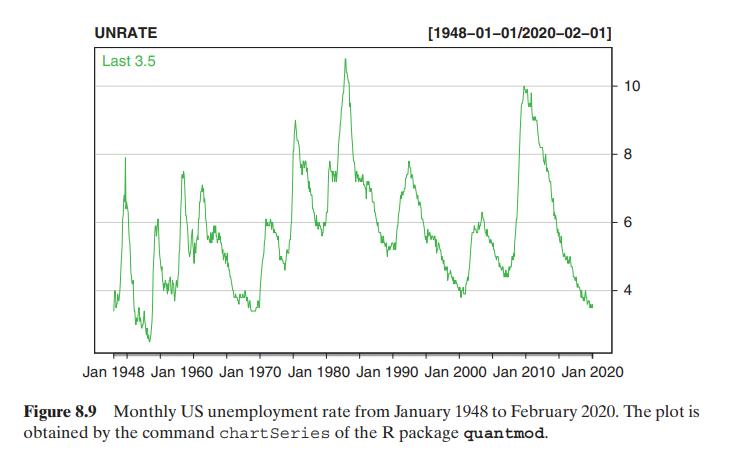
In this example, we consider US monthly unemployment rate from January 1948 to February 2020. The data are seasonally adjustment and can be downloaded directly from the FRED, which is the Economic Database of the Federal Reserve Banks at St. Louis. In fact, one can download the data over the Internet via the R package quantmod. Details are given in the attached R commands and output. Alternatively, the data are also in the file unrate4820.txt. Figure 8.9 shows the time plot of the US monthly unemployment rate data.

Example 8.3:

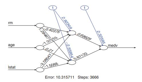
A widely used data set in the statistical literature is the Boston housing data set, which is available from the R package MASS. See Belsley et al. (2005) for a careful analysis of the data set. Here we use the data set only as an illustration. The dependent variable of interest is the median value of owner-occupied homes (in thousands)
of Boston suburbs. There are 13 predictors including rm (average number of rooms per dwelling), age (proportion of owner-occupied units built prior to 1940), and lstat (lower status of the population in percent). Our goal here is to demonstrate the use of NN so we only consider the aforementioned three predictors in the following analysis.
To begin, we take the log transformation of the dependent variable medv and standardize the input variables so that each of the predictor has mean 0 and variance 1. We then employ two NN models. The first model is a 3-2-1 network, which has 3 input variables, 1 single hidden layer with 2 nodes, and 1 output variable. Figure 8.6 displays the resulting network, where each numerical value associated with an arrow denotes the weight and the value associated with the arrow coming out of circle 1 denotes the bias. We use the default option so that the activation function is the logistic function. In this particular instance, the first node of the hidden layer is given by

\(h_1\left(\boldsymbol{x}_t\right)=\frac{\exp \left(2.923-0.404 \mathrm{rm}_t-1.373 \mathrm{age}_t-2.08 \text { lstat }_t\right)}{1+\exp \left(2.923-0.404 \mathrm{rm}_t-1.373 \mathrm{age}_t-2.08 \mathrm{lstat}_t\right)}\),

and the output node is 

\(\widehat{\operatorname{medv}}_t=2.326+0.686 h_1\left(\boldsymbol{x}_t\right)+0.871 h_2\left(\boldsymbol{x}_t\right)\).

Figure 8.6:

Transcribed Image Text:

UNRATE [1948-01-01/2020-02-01] Last 3.5 10 8 6 Jan 1948 Jan 1960 Jan 1970 Jan 1980 Jan 1990 Jan 2000 Jan 2010 Jan 2020 Figure 8.9 Monthly US unemployment rate from January 1948 to February 2020. The plot is obtained by the command chart Series of the R package quantmod.