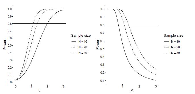
Consider Figure 4.2 and the $\mathrm{R}$ code that generated the plots. a. Modify the code so that sample size is on the $\mathrm{x}$-axis, and three different lines show the relationships between sample size and power for a difference of $\theta=1,2,3$. Fix the standard deviation to 1.5 for all lines.

b. Interpret the relationships between power, effect size $\theta$, standard deviation $\sigma$, and sample size $n$, on Figure 4.2 and the figure from part a. For example, what happens to power as $\theta$ decreases with $n$ and $\sigma$ fixed? How does $\theta$ change as power increases with other parameters fixed?

Data from Figure 4.2

Transcribed Image Text:

Power 1.0- 0.9- 0.8 0.7- 0.6- 0.5- 0.4- 0.3- 0.2 0.1- 0.0 1.0- 0.9- 0.8- 0.7- Sample size - N=10 0.6 - N=20 0.5- --- N = 30 0.4- 0.3- 0.2- 0.1 b Sample size - N = 10 - N=20 --- N=30