The following nonlinear differential equation was solved in Examples 24.4 and 24.7.

Such equations are sometimes linearized to obtain an approximate solution. This is done by employing a first-order Taylor series expansion to linearize the quartic term in the equation as

where T is a base temperature about which the term is linearized. Substitute this relationship into Eq. (P24.5), and then solve the resulting linear equation with the finite difference approach. Employ T = 300, Δx = 1m, and the parameters from Example 24.4 to obtain your solution. Plot your results along with those obtained for the nonlinear versions in Examples 24.4 and 24.7.

In Example 24.4:

Although it served our purposes for illustrating the shooting method, Eq. (24.6) was not a completely realistic model for a heated rod. For one thing, such a rod would lose heat by mechanisms such as radiation that are nonlinear.

Suppose that the following nonlinear ODE is used to simulate the temperature of the heated rod:

where σ′ = a bulk heat-transfer parameter reflecting the relative impacts of radiation and conduction = 2.7 × 10⁻⁹ K⁻³ m⁻² . This equation can serve to illustrate how the shooting method is used to solve a two-point nonlinear boundary-value problem. The remaining problem conditions are as specified in Example 24.2: L = 10 m, h′ = 0.05 m⁻² , T_∞ = 200 K, T(0) = 300 K, and T(10) = 400 K.

In Example 24.7:

Use the finite-difference approach to simulate the temperature of a heated rod subject to both convection and radiation:

where σ′ = 2.7 × 10⁻⁹ K⁻³m⁻² , L = 10 m, h′ = 0.05 m⁻² ,T_∞ = 200 K,T(0) = 300 K, andT(10) = 400 K. Use four interior nodes with a segment length of Δx = 2 m.

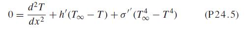
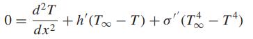
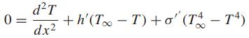
0= +h' (ToT) +o' (T - T4) dT dx (P24.5)