Project the 2^4-1_IV design in Example 8-1 into two replicates of a 2² design in the factors A and B. Analyze the data and thaw conclusions.

Example 8-1:

Consider the filtration rate experiment in Example 6.2. The original design, shown in Table 6.10, is a single replicate of the 2⁴ design. In that example, we found that the main effects A, C, and D and the interactions AC and AD were different from zero. We will now return to this experiment and simulate what would have happened if a half-fraction of the 2⁴ design had been run instead of the full factorial.

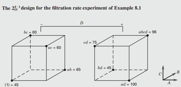
We will use the 2^4−1 design with I = ABCD, because this choice of generator will result in a design of the highest possible resolution (IV). To construct the design, we first write down the basic design, which is a 2₃ design, as shown in the first three columns of Table 8.3. This basic design has the necessary number of runs (eight) but only three columns (factors). To find the fourth factor levels, solve I = ABCD for D, or D = ABC. Thus, the level of D in each run is the product of the plus and minus signs in columns A, B, and C. The process is illustrated in Table 8.3. Because the generator ABCD is positive, this design is the principal fraction. The design is shown graphically in Figure 8.3.

Using the defining relation, we note that each main effect is aliased with a three-factor interaction; that is, A = A²BCD = BCD, B = AB²CD = ACD, C = ABC²D =ABD, and D = ABCD² = ABC. Furthermore, every two-factor interaction is aliased with another two-factor interaction. These alias relationships are AB = CD, AC = BD, and BC = AD. The four main effects plus the three two-factor interaction alias pairs account for the seven degrees of freedom for the design.

TABLE 8.3:

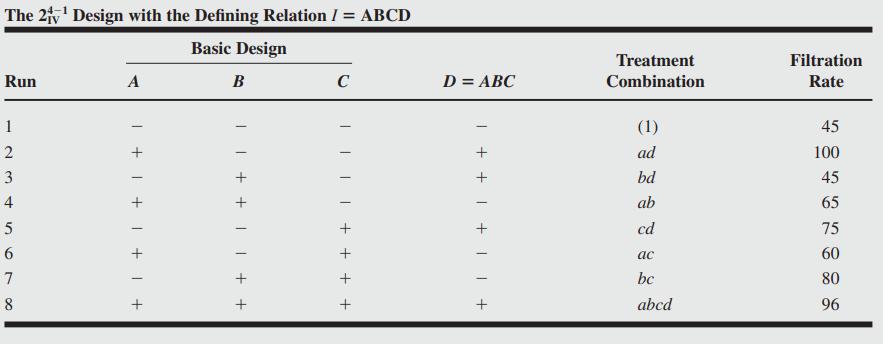
At this point, we would normally randomize the eight runs and perform the experiment. Because we have already run the full 2⁴ design, we will simply select the eight observed filtration rates from Example 6.2 that correspond to the runs in the design. These observations are shown in the last column of Table 8.3 as well as in Figure 8.3.

The estimates of the effects obtained from this 2^4−1_IV design are shown in Table 8.4. To illustrate the calculations, the linear combination of observations associated with the A effect is

whereas for the AB effect, we would obtain

From inspection of the information in Table 8.4, it is not unreasonable to conclude that the main effects A, C, and D are large. The AB + CD alias chain has a small estimate, so the simplest interpretation is that both the AB and CD interactions are negligible (otherwise, both AB and CD are large, but they have nearly identical magnitudes and opposite signs—this is fairly unlikely). Furthermore, if A, C, and D are the important main effects, then it is logical to conclude that the two interaction alias chains AC + BD and AD + BC have large effects because the AC and AD interactions are also significant. In other words, if A, C, and D are significant then the significant interactions are most likely AC and AD. This is an application of Ockham’s razor (after William of Ockham), a scientific principle that when one is confronted with several different possible interpretations of a phenomena, the simplest interpretation is usually the correct one. Note that this interpretation agrees with the conclusions from the analysis of the complete 2⁴ design in Example 6.2.

FIGURE 8.3:

Another way to view this interpretation is from the standpoint of effect heredity. Suppose that AB is significant and that both main effects A and B are significant. This is called strong heredity, and it is the usual situation (if an intraction is significant and only one of the main effects is significant this is called weak heredity; and this is relatively less common). So in this example, with A significant and B not significant this support the assumption that AB is not significant.

TABLE 8.4:

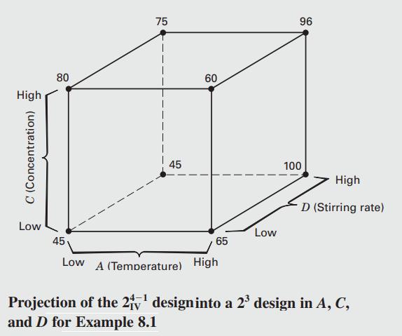
Because factor B is not significant, we may drop it from consideration. Consequently, we may project this 2^4−1_IV design into a single replicate of the 2³ design in factors A, C, and D, as shown in Figure 8.4. Visual examination of this cube plot makes us more comfortable with the conclusions reached above. Notice that if the temperature (A) is at the low level, the concentration (C) has a large positive effect, whereas if the temperature is at the high level, the concentration has a very small effect. This is probably due to an AC interaction. Furthermore, if the temperature is at the low level, the effect of the stirring rate (D) is negligible, whereas if the temperature is at the high level, the stirring rate has a large positive effect. This is probably due to the AD interaction tentatively identified previously.

Based on the above analysis, we can now obtain a model to predict filtration rate over the experimental region. This model is

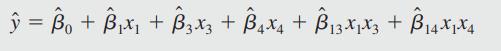
FIGURE 8.4:

where x₁, x₃, and x₄ are coded variables (−1 ≤ x_i ≤ +1) that represent A, C, and D, and the β̂'s are regression coefficients that can be obtained from the effect estimates as we did previously. Therefore, the prediction equation is

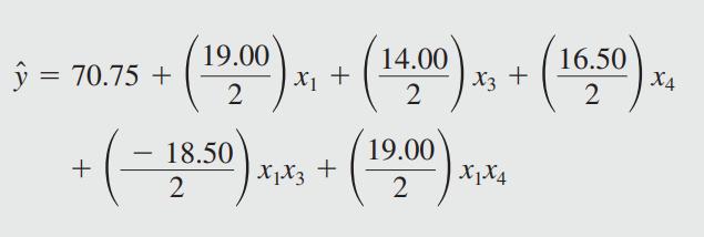
Remember that the intercept is the average of all responses at the eight runs in the design. This model is very similar to the one that resulted from the full 2^k factorial design in Example 6.2.

Example 6.2:

A chemical product is produced in a pressure vessel. A factorial experiment is carried out in the pilot plant to study the factors thought to influence the filtration rate of this product. The four factors are temperature (A), pressure (B), concentration of formaldehyde (C), and stirring rate (D). Each factor is present at two levels. The design matrix and the response data obtained from a single replicate of the 2⁴ experiment are shown in Table 6.10 and Figure 6.10. The 16 runs are made in random order. The process engineer is interested in maximizing the filtration rate. Current process conditions give filtration rates of around 75 gal/h. The process also currently uses the concentration of formaldehyde, factor C, at the high level. The engineer would like to reduce the formaldehyde concentration as much as possible but has been unable to do so because it always results in lower filtration rates.

TABLE 6.10:

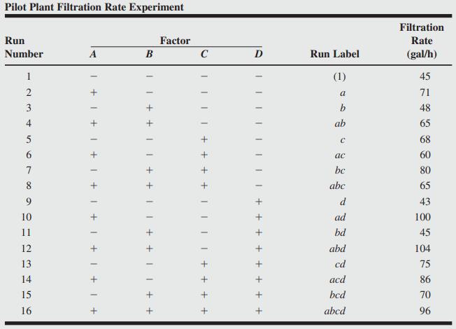
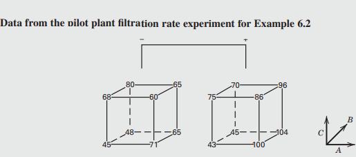
FIGURE 6.10:

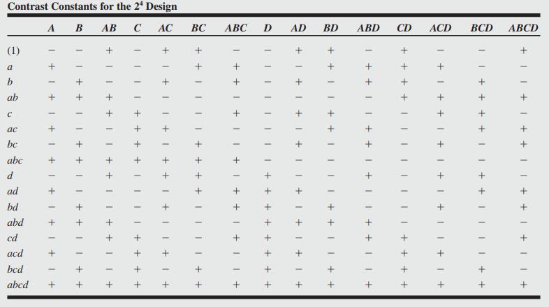
We will begin the analysis of these data by constructing a normal probability plot of the effect estimates. The table of plus and minus signs for the contrast constants for the 2⁴ design are shown in Table 6.11. From these contrasts, we may estimate the 15 factorial effects and the sums of squares shown in Table 6.12.

Table 6.11:

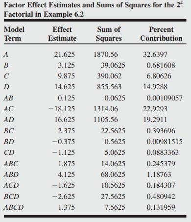
Table 6.12:

The normal probability plot of these effects is shown in Figure 6.11. All of the effects that lie along the line are negligible, whereas the large effects are far from the line. The important effects that emerge from this analysis are the main effects of A, C, and D and the AC and AD interactions.

The main effects of A, C, and D are plotted in Figure 6.12a. All three effects are positive, and if we considered only these main effects, we would run all three factors at the high level to maximize the filtration rate. However, it is always necessary to examine any interactions that are important. Remember that main effects do not have much meaning when they are involved in significant interactions.

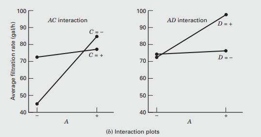
The AC and AD interactions are plotted in Figure 6.12b. These interactions are the key to solving the problem. Note from the AC interaction that the temperature effect is very small when the concentration is at the high level and very large when the concentration is at the low level, with the best results obtained with low concentration and high temperature. The AD interaction indicates that stirring rate D has little effect at low temperature but a large positive effect at high temperature. Therefore, the best filtration rates would appear to be obtained when A and D are at the high level and C is at the low level. This would allow the reduction of the formaldehyde concentration to a lower level, another objective of the experimenter

FIGURE 6.11 Normal probability plot of the effects for the 24 factorial in Example 6.2:

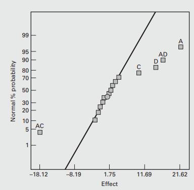
FIGURE 6.12a Main effect and interaction plots for Example 6.2:

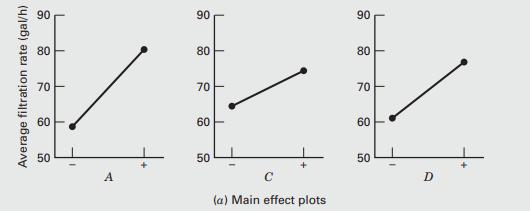
FIGURE 6.12b Main effect and interaction plots for Example 6.2: